| Python数据分析基础之描述性统计与建模(1) | 您所在的位置:网站首页 › python的描述性统计 › Python数据分析基础之描述性统计与建模(1) |
Python数据分析基础之描述性统计与建模(1)
|
葡萄酒质量数据集
葡萄酒质量数据集包括两个文件——红葡萄酒文件和白葡萄酒文件。红葡萄酒文件中包含1599条观测,白葡萄酒文件包含4898条观测。两个文件中都有1个输出变量和11个输入变量。输出变量是酒的质量,是一个从0(低质量)到10(高质量)的评分。输入变量是葡萄酒的物理化学成分和特性,包括非挥发性酸、挥发性酸、柠檬酸、残余糖分、氯化物、游离二氧化硫、总二氧化硫、密度、pH值、硫酸盐和酒精含量。 我们把这两个数据集合成一个数据集,保存在文件winequality-both.csv中。这个数据集中应该包括一个标题行和6497条。另外,还应该再添加一列,用来区分这行数据是红葡萄酒还是白葡萄酒的数据。 想要下载数据集?点我! 我们来对这个数据集进行分析。首先,我们要计算出每列的总体描述性统计量、质量列中的唯一值以及和这个唯一值对应的观测数量。代码如下: #!/usr/bin/env python3 import numpy as np import pandas as pd import seaborn as sns import matplotlib.pyplot as plt import statsmodels.api as sm import statsmodels.formula.api as smf from statsmodels.formula.api import ols, glm # 将数据集读入到pandas数据框中 wine = pd.read_csv('winequality-both.csv', sep=',', header=0) wine.columns = wine.columns.str.replace(' ', '_') print(wine.head()) # 显示所有变量的描述性统计量 print(wine.describe()) # 找出唯一值 print(sorted(wine.quality.unique())) # 计算值的频率 print(wine.quality.value_counts())在使用pandas模块的read_csv()方法将文本文件读入一个pandas数据框之后,我们使用head()函数检查一下标题行和前五行数据,确保数据被正确加载。第17行代码使用pandas的describe()函数打印出数据集中每个数值型变量的摘要统计量。第20行代码使用unique()识别出质量列中的唯一值,并以升序打印在屏幕上。最后,第23行代码计算出质量列中每个唯一值在数据集中出现的次数,并把它们以降序打印到屏幕上。 这段代码的运行结果如下: type fixed_acidity volatile_acidity ... sulphates alcohol quality 0 red 7.4 0.70 ... 0.56 9.4 5 1 red 7.8 0.88 ... 0.68 9.8 5 2 red 7.8 0.76 ... 0.65 9.8 5 3 red 11.2 0.28 ... 0.58 9.8 6 4 red 7.4 0.70 ... 0.56 9.4 5 [5 rows x 13 columns] fixed_acidity volatile_acidity ... alcohol quality count 6497.000000 6497.000000 ... 6497.000000 6497.000000 mean 7.215307 0.339666 ... 10.491801 5.818378 std 1.296434 0.164636 ... 1.192712 0.873255 min 3.800000 0.080000 ... 8.000000 3.000000 25% 6.400000 0.230000 ... 9.500000 5.000000 50% 7.000000 0.290000 ... 10.300000 6.000000 75% 7.700000 0.400000 ... 11.300000 6.000000 max 15.900000 1.580000 ... 14.900000 9.000000 [8 rows x 12 columns] [3, 4, 5, 6, 7, 8, 9] 6 2836 5 2138 7 1079 4 216 8 193 3 30 9 5 Name: quality, dtype: int64输出显示,质量评分中有6497个观测,评分范围从3到9,平均质量评分为5.8,标准差为0.87;质量列中的唯一值是3、4、5、6、7、8和9;有2836个观测的质量评分为6,2138个观测的质量评分为5,1079个观测的质量评分为7,216个观测的质量评分为4,193个观测的质量评分为8,30个观测的质量评分为3,5个观测的质量评分为9。 分组、直方图与t检验下面我们分别分析红葡萄酒数据和白葡萄酒数据,看看统计量是否会保持不变。 ... # 按照葡萄酒类型显示质量的描述性统计量 print(wine.groupby('type')[['quality']].describe().unstack('type')) # 按照葡萄酒类型显示质量的特定分位数值 print(wine.groupby('type')[['quality']].quantile([0.25, 0.75]).unstack('type')) # 按照葡萄酒类型查看质量分布 red_wine = wine.loc[wine['type'] == 'red', 'quality'] white_wine = wine.loc[wine['type'] == 'white', 'quality'] sns.set_style("dark") print(sns.distplot(red_wine, norm_hist=True, kde=False, color="red", label="Red wine")) print(sns.distplot(white_wine, norm_hist=True, kde=False, color="white", label="White wine")) sns.utils.axlabel("Quality Score", "Density") plt.title("Distribution of Quality by Wine Type") plt.legend() plt.show() # 检验红葡萄酒和白葡萄酒的平均质量是否有所不同 print(wine.groupby(['type'])[['quality']].agg(['std'])) tstat, pvalue, df = sm.stats.ttest_ind(red_wine, white_wine) print('tstat: %.3f pvalue: %.4f' % (tstat, pvalue))groupby()函数使用type列中的两个值将数据分为两组。方括号可以生成一个列表,列表中的元素是用来生成输出的列。在这里我们只对质量列应用describe()函数。这些命令的结果就是生成一列统计量,来自红葡萄酒数据的计算结果和白葡萄酒数据的计算结果是相互垂直地堆叠在一起的。unstack()函数将结果重新排列,这样红葡萄酒和白葡萄酒的统计量就会显示在并排的两列中。quantile()函数对质量列计算第25百分位数和第75百分位数。 接下来,我们使用seaborn创建直方图,红条表示红葡萄酒,白条表示白葡萄酒。因为白葡萄酒数据比红葡萄酒多,所以直方图显示密度分布而不是频率分布。 最后,进行一下t检验,判断红葡萄酒和白葡萄酒的平均评分是否有区别。在这里我们想知道红葡萄酒和白葡萄酒评分的标准差是否相同,所以在t检验中可以使用合并方差。 下面是这段代码的运行结果。 type quality count red 1599.000000 white 4898.000000 mean red 5.636023 white 5.877909 std red 0.807569 white 0.885639 min red 3.000000 white 3.000000 25% red 5.000000 white 5.000000 50% red 6.000000 white 6.000000 75% red 6.000000 white 6.000000 max red 8.000000 white 9.000000 dtype: float64 quality type red white 0.25 5.0 5.0 0.75 6.0 6.0 AxesSubplot(0.125,0.11;0.775x0.77) AxesSubplot(0.125,0.11;0.775x0.77) quality std type red 0.807569 white 0.885639 tstat: -9.686 pvalue: 0.0000
前面已经检查了输出变量,下面简单研究一下输入变量。让我们计算一下输入变量两两之间的相关性,并为一些输入变量创建带有回归直线的散点图: ... # 计算所有变量的相关矩阵 print(wine.corr()) # 从红葡萄酒和白葡萄酒的数据中取出一个“小”样本来进行绘图 def take_sample(data_frame, replace=False, n=200): return data_frame.loc[np.random.choice(data_frame.index, replace=replace, size=n)] reds_sample = take_sample(wine.loc[wine['type'] == 'red', :]) whites_sample = take_sample(wine.loc[wine['type'] == 'white', :]) wine_sample = pd.concat([reds_sample, whites_sample]) wine['in_sample'] = np.where(wine.index.isin(wine_sample.index), 1., 0.) print(pd.crosstab(wine.in_sample, wine.type, margins=True)) # 查看成对变量之间的关系 sns.set_style("dark") g = sns.pairplot(wine_sample, kind='reg', plot_kws={"ci": False, "x_jitter": 0.25, "y_jitter": 0.25}, hue='type', diag_kind='hist', diag_kws={"bins": 10, "alpha": 1.0}, palette=dict(red="red", white="white"), markers=["o", "s"], vars=['quality', 'alcohol', 'residual_sugar']) print(g) plt.suptitle('Histograms and Scatter Plots of Quality, Alcohol, and Residual Sugar', fontsize=14, horizontalalignment='center', verticalalignment='top', x=0.5, y=0.999) plt.show()corr()函数可以计算出数据集中所有变量两两之间的线性相关性。 数据集中有6000多个点,所以如果将它们都画在统计图中,就很难分辨出清楚的点。我们定义了一个函数take_sample(),用来抽取在统计图中使用的样本点。这个函数使用pandas数据框索引和numpy的random.choice()函数随机选择一个行的子集。我们是用这个函数对红葡萄酒和白葡萄酒分别进行抽样,并将抽样所得的两个数据框连接成一个数据框。然后,在wine数据框中创建一个新列in_sample,并使用numpy的where()函数和pandas的isin()函数对这个新列进行填充,填充的值根据此行的索引值是否在抽样数据的索引值中分别设为1和0.最后,我们使用pandas的crosstab()函数来确认in_sample列中包含400个1(200条红葡萄酒数据和200条白葡萄酒数据)和6097个0。 seaborn的pairplot()函数可以创建一个统计图矩阵。主对角线上的图以直方图或密度图的形式显示了每个变量的单变量分布,对角线之外的图以散点图的形式显示了每两个变量之间的双变量分布,散点图中可以有回归直线,也可以没有。因为质量评分都是整数,所以加上一点振动可以更容易看出数据在何处集中。 这段代码的运行结果如下: fixed_acidity volatile_acidity ... alcohol quality fixed_acidity 1.000000 0.219008 ... -0.095452 -0.076743 volatile_acidity 0.219008 1.000000 ... -0.037640 -0.265699 citric_acid 0.324436 -0.377981 ... -0.010493 0.085532 residual_sugar -0.111981 -0.196011 ... -0.359415 -0.036980 chlorides 0.298195 0.377124 ... -0.256916 -0.200666 free_sulfur_dioxide -0.282735 -0.352557 ... -0.179838 0.055463 total_sulfur_dioxide -0.329054 -0.414476 ... -0.265740 -0.041385 density 0.458910 0.271296 ... -0.686745 -0.305858 pH -0.252700 0.261454 ... 0.121248 0.019506 sulphates 0.299568 0.225984 ... -0.003029 0.038485 alcohol -0.095452 -0.037640 ... 1.000000 0.444319 quality -0.076743 -0.265699 ... 0.444319 1.000000 [12 rows x 12 columns] type red white All in_sample 0.0 1399 4698 6097 1.0 200 200 400 All 1599 4898 6497
相关系数和两两变量之间的统计图有助于对两个变量之间的关系进行量化和可视化,但是它们不能测量出每个自变量在其他自变量不变时与因变量之间的关系。线性回归可以解决这个问题。 线性回归模型如下: y i ∼ N ( μ i , σ 2 ) , y_i\sim N(\mu_i,\sigma^2), yi∼N(μi,σ2), μ i = β 0 + β 1 x i 1 + β 2 x i 2 + … + β p x i p \mu_i=\beta_0+\beta_1x_{i1}+\beta_2x_{i2}+…+\beta_px_{ip} μi=β0+β1xi1+β2xi2+…+βpxip对于 i = 1 , 2 , … , n i=1,2,…,n i=1,2,…,n个观测和 p p p个自变量。 这个模型表示观测 y i y_i yi服从均值为 μ i \mu_i μi方差为 σ 2 \sigma^2 σ2的正态分布(高斯分布),其中 μ i \mu_i μi依赖于自变量, σ 2 \sigma^2 σ2为一个常数。也就是说,给定了自变量的值之后,我们就可以得到一个具体的质量评分,但在另一天,给定同样的自变量值,我们可能会得到一个和前面不同的质量评分。但是,经过很多天自变量取同样的值(也就是一个很长的周期),质量评分会落在 μ i ± σ \mu_i±\sigma μi±σ这个范围内。 下面我们使用statsmodel包来进行线性回归: my_formula = 'quality ~ alcohol + chlorides + citric_acid + density +fixed_acidity + free_sulfur_dioxide + pH' \ '+ residual_sugar + sulphates + total_sulfur_dioxide + volatile_acidity' lm = ols(my_formula, data=wine).fit() # 或者,也可以使用广义线性模型(glm)语法进行线性回归 # lm = glm(my_formula, data=wine, family=sm.families.Gaussian()).fit() print(lm.summary()) print("\nQuantities you can extract from the result:\n%s" % dir(lm)) print("Coefficients:\n%s" % lm.params) print("Coefficient Std Errors:\n%s" % lm.bse) print("\nAdj. R-squared:\n%.2f" % lm.rsquared_adj) print("\nF-statistic: %.1f P-value: %.2f" % (lm.fvalue, lm.f_pvalue)) print("\nNumber of obs: %d Number of fitted values: %d" % (lm.nobs, len(lm.fittedvalues)))运行结果如下: OLS Regression Results ============================================================================== Dep. Variable: quality R-squared: 0.292 Model: OLS Adj. R-squared: 0.291 Method: Least Squares F-statistic: 243.3 Date: Thu, 27 Feb 2020 Prob (F-statistic): 0.00 Time: 23:03:10 Log-Likelihood: -7215.5 No. Observations: 6497 AIC: 1.445e+04 Df Residuals: 6485 BIC: 1.454e+04 Df Model: 11 Covariance Type: nonrobust ======================================================================================== coef std err t P>|t| [0.025 0.975] ---------------------------------------------------------------------------------------- Intercept 55.7627 11.894 4.688 0.000 32.447 79.079 alcohol 0.2670 0.017 15.963 0.000 0.234 0.300 chlorides -0.4837 0.333 -1.454 0.146 -1.136 0.168 citric_acid -0.1097 0.080 -1.377 0.168 -0.266 0.046 density -54.9669 12.137 -4.529 0.000 -78.760 -31.173 fixed_acidity 0.0677 0.016 4.346 0.000 0.037 0.098 free_sulfur_dioxide 0.0060 0.001 7.948 0.000 0.004 0.007 pH 0.4393 0.090 4.861 0.000 0.262 0.616 residual_sugar 0.0436 0.005 8.449 0.000 0.033 0.054 sulphates 0.7683 0.076 10.092 0.000 0.619 0.917 total_sulfur_dioxide -0.0025 0.000 -8.969 0.000 -0.003 -0.002 volatile_acidity -1.3279 0.077 -17.162 0.000 -1.480 -1.176 ============================================================================== Omnibus: 144.075 Durbin-Watson: 1.646 Prob(Omnibus): 0.000 Jarque-Bera (JB): 324.712 Skew: -0.006 Prob(JB): 3.09e-71 Kurtosis: 4.095 Cond. No. 2.49e+05 ============================================================================== Warnings: [1] Standard Errors assume that the covariance matrix of the errors is correctly specified. [2] The condition number is large, 2.49e+05. This might indicate that there are strong multicollinearity or other numerical problems. Quantities you can extract from the result: ['HC0_se', 'HC1_se', 'HC2_se', 'HC3_se', '_HCCM', '__class__', '__delattr__', '__dict__', '__dir__', '__doc__', '__eq__', '__format__', '__ge__', '__getattribute__', '__gt__', '__hash__', '__init__', '__init_subclass__', '__le__', '__lt__', '__module__', '__ne__', '__new__', '__reduce__', '__reduce_ex__', '__repr__', '__setattr__', '__sizeof__', '__str__', '__subclasshook__', '__weakref__', '_cache', '_data_attr', '_get_robustcov_results', '_is_nested', '_wexog_singular_values', 'aic', 'bic', 'bse', 'centered_tss', 'compare_f_test', 'compare_lm_test', 'compare_lr_test', 'condition_number', 'conf_int', 'conf_int_el', 'cov_HC0', 'cov_HC1', 'cov_HC2', 'cov_HC3', 'cov_kwds', 'cov_params', 'cov_type', 'df_model', 'df_resid', 'diagn', 'eigenvals', 'el_test', 'ess', 'f_pvalue', 'f_test', 'fittedvalues', 'fvalue', 'get_influence', 'get_prediction', 'get_robustcov_results', 'initialize', 'k_constant', 'llf', 'load', 'model', 'mse_model', 'mse_resid', 'mse_total', 'nobs', 'normalized_cov_params', 'outlier_test', 'params', 'predict', 'pvalues', 'remove_data', 'resid', 'resid_pearson', 'rsquared', 'rsquared_adj', 'save', 'scale', 'ssr', 'summary', 'summary2', 't_test', 't_test_pairwise', 'tvalues', 'uncentered_tss', 'use_t', 'wald_test', 'wald_test_terms', 'wresid'] Coefficients: Intercept 55.762750 alcohol 0.267030 chlorides -0.483714 citric_acid -0.109657 density -54.966942 fixed_acidity 0.067684 free_sulfur_dioxide 0.005970 pH 0.439296 residual_sugar 0.043559 sulphates 0.768252 total_sulfur_dioxide -0.002481 volatile_acidity -1.327892 dtype: float64 Coefficient Std Errors: Intercept 11.893899 alcohol 0.016728 chlorides 0.332683 citric_acid 0.079619 density 12.137473 fixed_acidity 0.015573 free_sulfur_dioxide 0.000751 pH 0.090371 residual_sugar 0.005156 sulphates 0.076123 total_sulfur_dioxide 0.000277 volatile_acidity 0.077373 dtype: float64 Adj. R-squared: 0.29 F-statistic: 243.3 P-value: 0.00 Number of obs: 6497 Number of fitted values: 6497字符串变量my_formula包含的是类似R语言语法的回归公式定义。波浪线左侧的变量quality是因变量,波浪线右侧的变量是自变量。 下一行代码使用公式和数据你喝一个普通最小二乘回归模型,并将结果赋给变量lm。被注释掉的那一行代码使用广义线性模型(glm)的语法代替普通最小二乘语法也可以拟合同样的模型。 Tips: dir():不带参数时,返回当前范围内的变量、方法和定义的类型列表;带参数时,返回参数的属性、方法列表 lm.params:以一个序列的形式返回模型系数 lm.rsquared_adj:返回修正R方 lm.fvalue:返回F统计量 lm.f_pvalue:返回F统计量的p值 lm.fittedvalues:返回拟合值 系数解释在这个模型中,某个自变量系数的意义是,在其他自变量保持不变的情况下,这个自变量发生1个单位的变化时,导致葡萄酒质量评分发生的平均变化。 并不是所有的系数都需要解释。例如,截距系数的意义是当所有自变量的值都为0时的期望评分。因为没有任何一种葡萄酒的各种成分都为0,所以截距系数没有具体意义。 自变量标准化关于这个模型,普通最小二乘回归是通过使残差平方和最小化来估计未知的 β \beta β参数值的,这里的残差是指自变量观测值与拟合值之间的差别。因为残差大小是依赖于自变量的测量单位的,所以如果自变量的测量单位相差很大的话,那么将自变量标准化后,就可以更容易对模型进行解释了。对自变量进行标准化的方法是,先从自变量的每个观测值中减去均值,然后再除以这个自变量的标准差。自变量标准化完成以后,它的均值为0,标准差为1。 在 Data Analysis Using Regression and Multilevel/Hierarchical Models (Cambridge University Press, 2007, p.56) 中,Gelman and Hill建议在数据集中既有连续型自变量又有二值型自变量的情况下,用两杯标准差去除,而不是用一倍标准差。这样的话,标准化自变量一个单位的变化就对应于均值上下一个标准差的变化。 ... # 创建一个名为dependent_variable的序列来保存质量数据 dependent_variable = wine['quality'] # 创建一个名为independent_variables的数据框来保存初始的葡萄酒数据集中除quality、type和in_sample之外的所有变量 independent_variables = wine[wine.columns.difference(['quality', 'type', 'in_sample'])] # 对自变量进行标准化 # 对每个变量,在每个观测中减去变量的均值 # 并且使用结果除以变量的标准差 independent_variables_standardized = (independent_variables - independent_variables.mean()) / independent_variables.std() # 将因变量quality作为一列添加到自变量数据框中 # 创建一个带有标准化自变量的新数据集 wine_standardized = pd.concat([dependent_variable, independent_variables_standardized], axis=1) # 重新进行线性回归,并查看一下摘要统计 lm_standardized = ols(my_formula, data=wine_standardized).fit() print(lm_standardized.summary())运行结果如下: OLS Regression Results ============================================================================== Dep. Variable: quality R-squared: 0.292 Model: OLS Adj. R-squared: 0.291 Method: Least Squares F-statistic: 243.3 Date: Fri, 28 Feb 2020 Prob (F-statistic): 0.00 Time: 16:31:15 Log-Likelihood: -7215.5 No. Observations: 6497 AIC: 1.445e+04 Df Residuals: 6485 BIC: 1.454e+04 Df Model: 11 Covariance Type: nonrobust ======================================================================================== coef std err t P>|t| [0.025 0.975] ---------------------------------------------------------------------------------------- Intercept 5.8184 0.009 637.785 0.000 5.800 5.836 alcohol 0.3185 0.020 15.963 0.000 0.279 0.358 chlorides -0.0169 0.012 -1.454 0.146 -0.040 0.006 citric_acid -0.0159 0.012 -1.377 0.168 -0.039 0.007 density -0.1648 0.036 -4.529 0.000 -0.236 -0.093 fixed_acidity 0.0877 0.020 4.346 0.000 0.048 0.127 free_sulfur_dioxide 0.1060 0.013 7.948 0.000 0.080 0.132 pH 0.0706 0.015 4.861 0.000 0.042 0.099 residual_sugar 0.2072 0.025 8.449 0.000 0.159 0.255 sulphates 0.1143 0.011 10.092 0.000 0.092 0.137 total_sulfur_dioxide -0.1402 0.016 -8.969 0.000 -0.171 -0.110 volatile_acidity -0.2186 0.013 -17.162 0.000 -0.244 -0.194 ============================================================================== Omnibus: 144.075 Durbin-Watson: 1.646 Prob(Omnibus): 0.000 Jarque-Bera (JB): 324.712 Skew: -0.006 Prob(JB): 3.09e-71 Kurtosis: 4.095 Cond. No. 9.61 ============================================================================== Warnings: [1] Standard Errors assume that the covariance matrix of the errors is correctly specified.自变量标准化会改变对模型系数的解释。现在每个自变量系数的含义是,不同的葡萄酒在其他自变量均相同的情况下,某个自变量相差1个标准差,会使葡萄酒的质量评分平均相差多少个标准差。 自变量标准化同样会改变对截距的解释。当解释变量被标准化后,截距表示的就是当所有自变量取值为均值时因变量的均值。 预测 ... # 使用葡萄酒数据集中的前10个观测创建10个“新”观测 # 新观测中只包含模型中使用的自变量 new_observations = wine.loc[wine.index.isin(range(10)), independent_variables.columns] # 基于新观测中的葡萄酒特性预测质量评分 y_predicted = lm.predict(new_observations) # 将预测值保留两位小数并打印到屏幕上 y_predicted_rounded = [round(score, 2) for score in y_predicted] print(y_predicted_rounded)运行结果如下: [5.0, 4.92, 5.03, 5.68, 5.0, 5.04, 5.02, 5.3, 5.24, 5.69] |

 由绘制的密度分布直方图和输出结果可以得出结论:两种葡萄酒的评分都近似正态分布;t检验统计量为-9.686,p值为0.000,这说明白葡萄酒的平均质量评分在统计意义上大于红葡萄酒的平均质量评分。
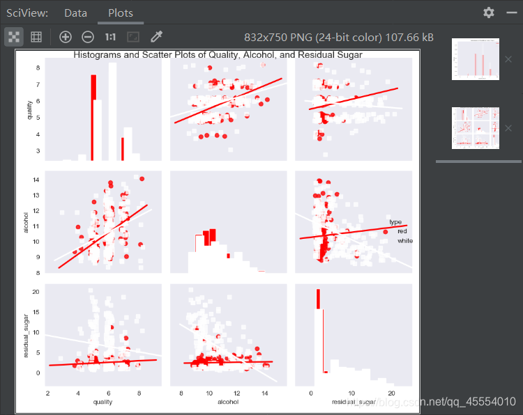 根据相关系数的符号,从输出中可以知道酒精含量、硫酸盐、pH值、游离二氧化硫和柠檬酸这些指标与质量是正相关的,相反,非挥发性酸、挥发性酸、残余糖分、氯化物、总二氧化硫和密度这些指标与质量是负相关的。 从统计图中可以看出,对于红葡萄酒和白葡萄酒来说,酒精含量的均值和标准差是大致相同的,但是,白葡萄酒残余糖分的均值和标准差却大于红葡萄酒残余糖分的均值和标准差。从回归直线可以看出,对于两种类型的葡萄酒,酒精含量增加时,质量评分也随之提高,相反,残余糖分增加时,质量评分则随之降低。这两个变量对白葡萄酒的影响都要大于对红葡萄酒的影响。
【本文地址】