| 2023年的深度学习入门指南(8) | 您所在的位置:网站首页 › 神经网络 剪枝率定义是什么 › 2023年的深度学习入门指南(8) |
2023年的深度学习入门指南(8)
|
2023年的深度学习入门指南(8) - 剪枝和量化
从这一节开始,我们要准备一些技术专项了。因为目前大模型技术还在快速更新迭代中,各种库和实现每天都在不停出现。因为变化快,所以难免会遇到一些问题。对于细节有一定的把握能力起码可以做到出问题不慌,大致知道从哪方面入手。 我们首先从如何优化大模型的大小,使其能够在更少计算资源的情况下运行起来。 针对模型太大,比较显而易见的是有三种思路: 有损或无损地对模型进行压缩:比如将不重要的网络节点和边去掉,这叫作剪枝;再如将16位浮点数运算变成8位整数运算,这叫作量化。采用更有效的学习算法。比如不是从原始数据中学习,而是跟大模型学,这叫做蒸馏。改进网络的结构,更有效发挥硬件能力等等。我们这一节先说模型压缩方法:剪枝和量化。 剪枝以全连接网络为例,网络都是节点和连接节点的边组成的。我们想要压缩网络的大小,就可以通过计算,将一些不重要的节点从图中删除掉,如下图所示:
这个算法出自名门,是神经网络获得图灵奖的三巨头之一的Yann LeCun于1989年就研究出来了。 比如我们可以取让损失函数变化最大的节点作为被剪掉的节点。也可以采用随机策略随机删掉一个节点。也可以根据网络的结构取中间层进行剪枝,以减少对节点较小的输入输出层的影响。随机剪枝我们也称之为非结构化剪枝,而按模块进行剪枝的称为结构化剪枝。 从剪掉的节点数量上考虑,既可以每一轮被剪掉均匀的数量,也可以开始的时候多剪一些,后面慢慢变少。 最后,如果剪过头影响性能了,我们还可以让部分节点重新生长出来。然后可以再次尝试下一轮剪枝。 在主要框架中,早已经集成好了剪枝功能,比如在PyTorch中,剪枝功能是在torch.nn.utils.prune中定义的。 我们先看L1Unstructured,它是取将最小的L1-Norm值的节点剪掉为策略的剪枝方法: import torch import torch.nn as nn import torch.nn.utils.prune as prune # 定义一个简单的神经网络 class SimpleNN(nn.Module): def __init__(self): super(SimpleNN, self).__init__() self.fc1 = nn.Linear(10, 5) self.fc2 = nn.Linear(5, 3) def forward(self, x): x = self.fc1(x) x = self.fc2(x) return x # 实例化网络 model = SimpleNN() # 使用 L1Unstructured 对第一个全连接层进行剪枝 # 剪枝前,查看权重 print("Before pruning:") print(model.fc1.weight) # 应用 L1Unstructured 剪枝方法,保留 50% 的权重 prune.l1_unstructured(model.fc1, name='weight', amount=0.5) # 剪枝后,查看权重 print("After pruning:") print(model.fc1.weight)我们来看看运行结果。剪枝之前的: Before pruning: Parameter containing: tensor([[ 0.1743, -0.1874, -0.1400, 0.1085, 0.0037, 0.2902, -0.0728, 0.2963, -0.1599, -0.1496], [-0.0496, -0.0954, 0.0030, -0.1801, 0.1881, 0.0244, 0.0629, -0.2639, -0.0755, -0.2218], [-0.2467, -0.1869, 0.0836, 0.0503, 0.2446, -0.2809, 0.1273, 0.0471, -0.1552, 0.0118], [-0.2023, -0.2786, -0.2742, 0.0381, -0.0608, 0.0737, -0.1440, -0.0835, -0.0172, 0.1741], [-0.1663, -0.1361, 0.2251, -0.1459, 0.1826, -0.1802, 0.2597, 0.2781, 0.1729, -0.1752]], requires_grad=True)剪枝之后的: After pruning: tensor([[ 0.1743, -0.1874, -0.0000, 0.0000, 0.0000, 0.2902, -0.0000, 0.2963, -0.1599, -0.0000], [-0.0000, -0.0000, 0.0000, -0.1801, 0.1881, 0.0000, 0.0000, -0.2639, -0.0000, -0.2218], [-0.2467, -0.1869, 0.0000, 0.0000, 0.2446, -0.2809, 0.0000, 0.0000, -0.0000, 0.0000], [-0.2023, -0.2786, -0.2742, 0.0000, -0.0000, 0.0000, -0.0000, -0.0000, -0.0000, 0.1741], [-0.1663, -0.0000, 0.2251, -0.0000, 0.1826, -0.1802, 0.2597, 0.2781, 0.1729, -0.1752]], grad_fn=)我们可以看到,一半的权重值已经被剪成0了。 我们也可以使用torch.nn.utils.prune.random_unstructured函数来实现随机剪枝: import torch import torch.nn as nn import torch.nn.utils.prune as prune # 定义一个简单的神经网络 class SimpleNN(nn.Module): def __init__(self): super(SimpleNN, self).__init__() self.fc1 = nn.Linear(10, 5) self.fc2 = nn.Linear(5, 3) def forward(self, x): x = self.fc1(x) x = self.fc2(x) return x # 实例化网络 model = SimpleNN() # 使用 random_unstructured 对第一个全连接层进行剪枝 # 剪枝前,查看权重 print("Before pruning:") print(model.fc1.weight) # 应用 random_unstructured 剪枝方法,保留 50% 的权重 prune.random_unstructured(model.fc1, name='weight', amount=0.5) # 剪枝后,查看权重 print("After pruning:") print(model.fc1.weight)随机剪枝的结果与上面的L1不同在于,每一次运行的结果是不相同的。 说完非结构化的,我们再来看结构化的。 结构化可以定义维,比如将第一维的都剪掉,我们看例子: import torch import torch.nn as nn import torch.nn.utils.prune as prune # 定义一个简单的神经网络 class SimpleNN(nn.Module): def __init__(self): super(SimpleNN, self).__init__() self.fc1 = nn.Linear(10, 10) self.fc2 = nn.Linear(10, 5) self.fc3 = nn.Linear(5, 3) def forward(self, x): x = self.fc1(x) x = self.fc2(x) x = self.fc3(x) return x # 实例化网络 model = SimpleNN() # 使用 L1Unstructured 对第一个全连接层进行剪枝 # 剪枝前,查看权重 print("Before pruning:") print(model.fc1.weight) # 应用 random_structured 剪枝方法,保留 50% 的权重 prune.random_structured(model.fc1, name='weight',amount=0.5, dim=1) # 剪枝后,查看权重 print("After pruning:") print(model.fc1.weight)我们来看运行结果: Before pruning: Parameter containing: tensor([[ 1.8203e-01, -2.4652e-02, -1.8870e-01, -2.0959e-01, -1.4791e-01, 1.7911e-01, 2.1782e-01, 2.0245e-01, -7.1234e-02, -2.4723e-01], [ 2.0795e-01, -2.4798e-01, -6.2147e-03, -2.7634e-01, -3.6599e-02, -1.2186e-01, -9.3189e-02, 1.0184e-01, 9.8952e-02, -1.6860e-01], [ 8.2882e-03, -9.2586e-02, 1.1309e-01, 1.3828e-01, 1.5534e-01, -6.5238e-02, -2.4512e-01, -1.8104e-01, -1.7913e-01, -6.7663e-02], [ 1.6401e-01, 1.5702e-01, -2.7113e-01, -1.1145e-01, -3.8372e-02, 1.9320e-01, -1.1800e-01, -1.6497e-03, -2.7625e-01, 2.4986e-01], [ 9.3429e-02, -1.9261e-01, 1.1799e-02, -3.1452e-01, 3.8984e-02, 2.5882e-01, 1.7893e-01, -3.0125e-01, 2.1812e-01, 3.0290e-01], [-9.5934e-05, -8.3178e-02, 1.2058e-01, -2.8590e-01, 2.9342e-01, -1.3845e-01, -2.2089e-01, -9.1614e-02, 2.7203e-01, -1.7542e-01], [ 1.5185e-02, -2.5059e-01, 2.8496e-01, 2.6329e-01, 8.1400e-02, 2.1947e-01, -2.0651e-01, 2.3151e-01, 2.5052e-01, 7.7183e-02], [-4.8820e-02, -7.7806e-02, -2.2073e-01, 5.1517e-03, -2.3736e-01, -1.4963e-01, -2.0640e-01, -1.7726e-01, -2.6281e-01, -6.7827e-02], [-6.8090e-02, 3.0740e-01, 3.0408e-01, 1.8012e-01, 8.3739e-02, -2.3268e-01, 2.1999e-02, 1.3235e-01, 4.1730e-03, 2.9417e-01], [-3.3793e-02, 2.4021e-01, -6.9832e-02, -2.7820e-01, -1.7553e-01, 9.3053e-02, -2.2394e-01, -2.2041e-01, 1.6536e-01, -6.8046e-02]], requires_grad=True) After pruning: tensor([[ 1.8203e-01, -0.0000e+00, -1.8870e-01, -2.0959e-01, -1.4791e-01, 1.7911e-01, 0.0000e+00, 0.0000e+00, -0.0000e+00, -0.0000e+00], [ 2.0795e-01, -0.0000e+00, -6.2147e-03, -2.7634e-01, -3.6599e-02, -1.2186e-01, -0.0000e+00, 0.0000e+00, 0.0000e+00, -0.0000e+00], [ 8.2882e-03, -0.0000e+00, 1.1309e-01, 1.3828e-01, 1.5534e-01, -6.5238e-02, -0.0000e+00, -0.0000e+00, -0.0000e+00, -0.0000e+00], [ 1.6401e-01, 0.0000e+00, -2.7113e-01, -1.1145e-01, -3.8372e-02, 1.9320e-01, -0.0000e+00, -0.0000e+00, -0.0000e+00, 0.0000e+00], [ 9.3429e-02, -0.0000e+00, 1.1799e-02, -3.1452e-01, 3.8984e-02, 2.5882e-01, 0.0000e+00, -0.0000e+00, 0.0000e+00, 0.0000e+00], [-9.5934e-05, -0.0000e+00, 1.2058e-01, -2.8590e-01, 2.9342e-01, -1.3845e-01, -0.0000e+00, -0.0000e+00, 0.0000e+00, -0.0000e+00], [ 1.5185e-02, -0.0000e+00, 2.8496e-01, 2.6329e-01, 8.1400e-02, 2.1947e-01, -0.0000e+00, 0.0000e+00, 0.0000e+00, 0.0000e+00], [-4.8820e-02, -0.0000e+00, -2.2073e-01, 5.1517e-03, -2.3736e-01, -1.4963e-01, -0.0000e+00, -0.0000e+00, -0.0000e+00, -0.0000e+00], [-6.8090e-02, 0.0000e+00, 3.0408e-01, 1.8012e-01, 8.3739e-02, -2.3268e-01, 0.0000e+00, 0.0000e+00, 0.0000e+00, 0.0000e+00], [-3.3793e-02, 0.0000e+00, -6.9832e-02, -2.7820e-01, -1.7553e-01, 9.3053e-02, -0.0000e+00, -0.0000e+00, 0.0000e+00, -0.0000e+00]], grad_fn=)大家看到那一列整齐的正0和负0了么。当然,这一维全0了,仍然不够50%,其他维还是要再出一些名额的。 量化在ARM处理器大核都要把32位计算模块砍掉的情况下,64位计算已经成为了哪怕是手机上的主流。最不济也可以使用32位的指令。在深度学习的计算中,我们主要使用也是32位精度的浮点计算。 当模型变大后,如果我们可以将32位浮点运算变成8位整数运算,甚至极端情况下搞成4位整数运算,则不管是在存储还是计算上都节省大量的资源。 量化的算法很容易想到,压缩时就是把一个区间的值都映射到一个离散值上。还原时就想办法恢复成之前的值。 最极端的情况下就是二值量化,这就退化成符号函数或者是激活函数了。
对照上图,量化要做的事情,就是尽可能有效地利用有限的量化后的存储空间,让原始数据的损失最小。 如果这么说比较抽象的话,我们边写代码,边举例子说明。 固定大小量化方法在PyTorch中,量化函数quantize_per_tensor主要需要三个参数:缩放因子,零点和量化类型。 类型我们取8位无符号数。 缩放因子的公式:scale = (max_val - min_val) / (qmax - qmin) 零点的计算公式:zero_point = qmin - round(min_val / scale) 对于8位无符号数的话,qmax = 256, qmin = 0。 我们先随便写一个找找感觉: import torch x = torch.rand(2, 3, dtype=torch.float32) print(x) xq = torch.quantize_per_tensor(x, scale=0.5, zero_point=0, dtype=torch.quint8) print(xq)如果想看到量化之后的整数表示,我们可以通过int_repr方法来查看。 xq.int_repr()最后,我们可以用dequantize来解量化: xd = xq.dequantize() print(xd)torch.rand是取0到1之间的浮点数,那么max_val为1.0,min_val为0.0. scale就是1/256. 我们把上面的串在一起: import torch x = torch.rand(2, 3, dtype=torch.float32) print(x) xq = torch.quantize_per_tensor(x, scale=1/256, zero_point=0, dtype=torch.quint8) print(xq) # 看整数的表示: print(xq.int_repr()) # 解量化 xd = xq.dequantize() print(xd)随机生成的值是这样的: tensor([[0.8779, 0.2919, 0.6965], [0.8018, 0.2809, 0.0910]])量化之后的值为整数值为: tensor([[225, 75, 178], [205, 72, 23]], dtype=torch.uint8)解量化之后的结果为: tensor([[0.8789, 0.2930, 0.6953], [0.8008, 0.2812, 0.0898]])基本上还是可以保证小数点之后两位左右的准确率。 如果我们还想省得更多,采用4位做量化会是什么样的结果呢? 4位的话,scale就变成1/16了: import torch x = torch.tensor([[0.8779, 0.2919, 0.6965], [0.8018, 0.2809, 0.0910]]) print(x) xq = torch.quantize_per_tensor(x, scale=1/16, zero_point=0, dtype=torch.quint8) print(xq) # 看整数的表示: print(xq.int_repr()) # 解量化 xd = xq.dequantize() print(xd)输出结果如下: tensor([[0.8779, 0.2919, 0.6965], [0.8018, 0.2809, 0.0910]]) tensor([[0.8750, 0.3125, 0.6875], [0.8125, 0.2500, 0.0625]], size=(2, 3), dtype=torch.quint8, quantization_scheme=torch.per_tensor_affine, scale=0.0625, zero_point=0) tensor([[14, 5, 11], [13, 4, 1]], dtype=torch.uint8) tensor([[0.8750, 0.3125, 0.6875], [0.8125, 0.2500, 0.0625]])可以看到,当只有4位量化的时候,只能做到1位小数差不多了。 自动调整区间的量化不过,观察上面的量化结果,我们发现,我们取的max_val和min_val都偏保守。 以上面4位量化为例: tensor([[14, 5, 11], [13, 4, 1]], dtype=torch.uint8)我们上没有用到15,下没有用到0,明显是浪费了一点精度。 为了更充分发挥潜力,我们可以计算更精确一些。 当然,这事情不需要手工搞,PyTorch为我们准备好了torch.quantization.MinMaxObserver,我们只要设定好范围,就可以调用calculate_qparams方法来自动计算缩放因子和零点位置: observer = torch.quantization.MinMaxObserver(quant_min=0,quant_max=15) observer(x) scale, zero_point = observer.calculate_qparams() print(scale, zero_point)跟上面的例子组合一下: import torch x = torch.tensor([[0.8779, 0.2919, 0.6965], [0.8018, 0.2809, 0.0910]]) print(x) observer = torch.quantization.MinMaxObserver(quant_min=0,quant_max=15) observer(x) scale, zero_point = observer.calculate_qparams() print(scale, zero_point) xq = torch.quantize_per_tensor(x, scale=scale, zero_point=zero_point, dtype=torch.quint8) print(xq) # 看整数的表示: print(xq.int_repr()) # 解量化 xd = xq.dequantize() print(xd)我们看一下结果: tensor([[0.8779, 0.2919, 0.6965], [0.8018, 0.2809, 0.0910]]) tensor([0.0585]) tensor([0], dtype=torch.int32) tensor([[0.8779, 0.2926, 0.7023], [0.8194, 0.2926, 0.1171]], size=(2, 3), dtype=torch.quint8, quantization_scheme=torch.per_tensor_affine, scale=0.058526668697595596, zero_point=0) tensor([[15, 5, 12], [14, 5, 2]], dtype=torch.uint8) tensor([[0.8779, 0.2926, 0.7023], [0.8194, 0.2926, 0.1171]])scale从0.0625降低到了0.058526668697595596,能提升6%吧。 更主要的是,随着可以使用动态监控,我们以后不管针对什么样的数据分布,都可以用更加符合大小的值来进行量化。 对了,在2023年4月20日这个时间点,PyTorch的量化功能还处于beta阶段。后面正式发布了我再更新。 量化的硬件支持经过上面的学习,我们对量化的原理和编程已经有了一个比较清晰的了解。 不过,在实际应用中并没有这么简单。在实际硬件中,如果是只有CPU的情况下,我们使用FBGEMM库来实现加速。 import torch # define a floating point model where some layers could be statically quantized class M(torch.nn.Module): def __init__(self): super().__init__() # QuantStub converts tensors from floating point to quantized self.quant = torch.ao.quantization.QuantStub() self.conv = torch.nn.Conv2d(1, 1, 1) self.relu = torch.nn.ReLU() # DeQuantStub converts tensors from quantized to floating point self.dequant = torch.ao.quantization.DeQuantStub() def forward(self, x): # manually specify where tensors will be converted from floating # point to quantized in the quantized model x = self.quant(x) x = self.conv(x) x = self.relu(x) # manually specify where tensors will be converted from quantized # to floating point in the quantized model x = self.dequant(x) return x # create a model instance model_fp32 = M() # model must be set to eval mode for static quantization logic to work model_fp32.eval() # attach a global qconfig, which contains information about what kind # of observers to attach. Use 'x86' for server inference and 'qnnpack' # for mobile inference. Other quantization configurations such as selecting # symmetric or asymmetric quantization and MinMax or L2Norm calibration techniques # can be specified here. # Note: the old 'fbgemm' is still available but 'x86' is the recommended default # for server inference. # model_fp32.qconfig = torch.ao.quantization.get_default_qconfig('fbgemm') model_fp32.qconfig = torch.ao.quantization.get_default_qconfig('x86') # Fuse the activations to preceding layers, where applicable. # This needs to be done manually depending on the model architecture. # Common fusions include `conv + relu` and `conv + batchnorm + relu` model_fp32_fused = torch.ao.quantization.fuse_modules(model_fp32, [['conv', 'relu']]) # Prepare the model for static quantization. This inserts observers in # the model that will observe activation tensors during calibration. model_fp32_prepared = torch.ao.quantization.prepare(model_fp32_fused) # calibrate the prepared model to determine quantization parameters for activations # in a real world setting, the calibration would be done with a representative dataset input_fp32 = torch.randn(4, 1, 4, 4) model_fp32_prepared(input_fp32) # Convert the observed model to a quantized model. This does several things: # quantizes the weights, computes and stores the scale and bias value to be # used with each activation tensor, and replaces key operators with quantized # implementations. model_int8 = torch.ao.quantization.convert(model_fp32_prepared) # run the model, relevant calculations will happen in int8 res = model_int8(input_fp32) print(res)如果是在手机上运行,就要使用qnnpack库来替换掉x86或者fbgemm: model_fp32.qconfig = torch.ao.quantization.get_default_qconfig('qnnpack')FBGEMM和qnnpack都是矩阵计算的加速库。 fbgemm库FBGEMM (Facebook’s Gemm Library) 是一个高性能、低精度矩阵乘法库,适用于服务器端的 x86 架构。它广泛应用于深度学习、推荐系统等领域。 我们来写个例子理解FBGEMM是什么。 先下载FBGEMM的代码: git clone --recursive https://github.com/pytorch/FBGEMM.git cd FBGEMM mkdir build && cd build cmake .. make make install为了可以编译成功,我们还需要一个BLAS库,比如使用Intel的MKL库,或者是OpenBLAS库。后面我们会详细介绍这些支持并行开发的库。 编译成功之后,我们写个调用fbgemm进行矩阵计算的例子: #include #include "fbgemm/Fbgemm.h" int main() { // 定义矩阵维度 int M = 3; int N = 2; int K = 4; // 定义矩阵 A 和 B float A[M * K] = {1, 2, 3, 4, 5, 6, 7, 8, 9, 10, 11, 12}; float B[K * N] = {1, 2, 3, 4, 5, 6, 7, 8}; // 初始化 C 矩阵 float C[M * N] = {0}; // 定义 FBGEMM 参数 fbgemm::matrix_op_t A_op = fbgemm::matrix_op_t::NoTranspose; fbgemm::matrix_op_t B_op = fbgemm::matrix_op_t::NoTranspose; // 执行矩阵乘法运算 fbgemm::cblas_sgemm_ref(M, N, K, A, K, A_op, B, N, B_op, C, N); // 打印结果矩阵 C std::cout std::cout |
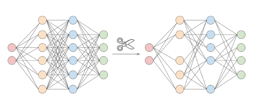
 剪枝虽然看起来简单粗暴,跟企业裁员似的。但是操作起来需要小火慢慢来的,一般在一个训练好的大网络上,一次一次迭代地将最低显著性分数的节点去掉,这样可以让损失变得最小化。 剪枝完成后,还要用剪完的网络进行微调,使得性能更好。 如果一次剪枝之后还达不到要求,这个过程可以重复多次,直到满足对于小模型的需求为止。
【本文地址】