通过核基本阈值分类器进行高光谱图像分类（Matlab代码实现）

 👨‍🎓个人主页：研学社的博客    

💥💥💞💞欢迎来到本博客❤️❤️💥💥

🏆博主优势：🌞🌞🌞博客内容尽量做到思维缜密，逻辑清晰，为了方便读者。

⛳️座右铭：行百里者，半于九十。

📋📋📋本文目录如下：🎁🎁🎁

目录

💥1 概述

📚2 运行结果

🎉3 参考文献

🌈4 Matlab代码实现

文献来源：

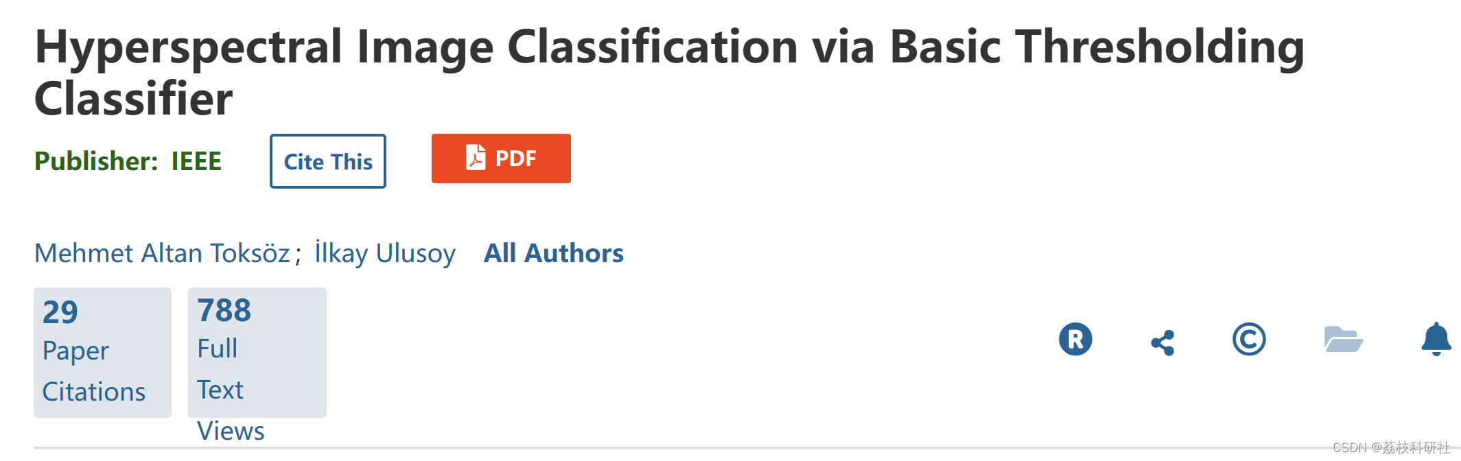
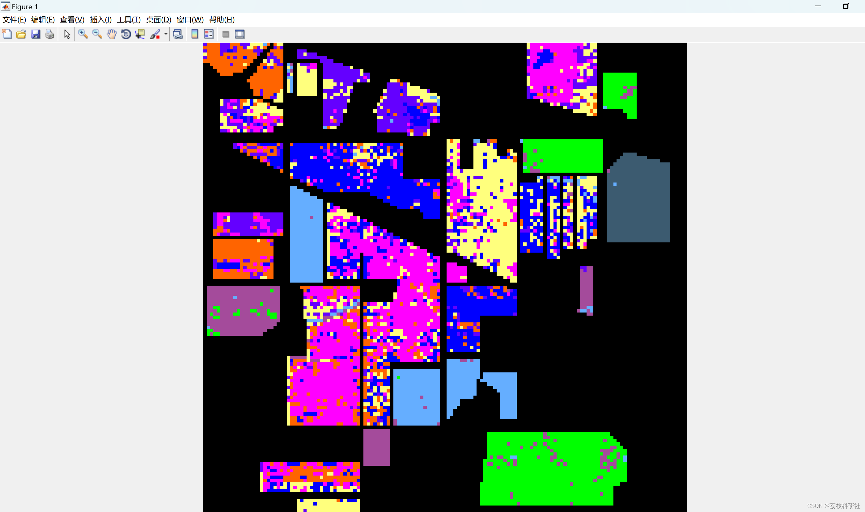
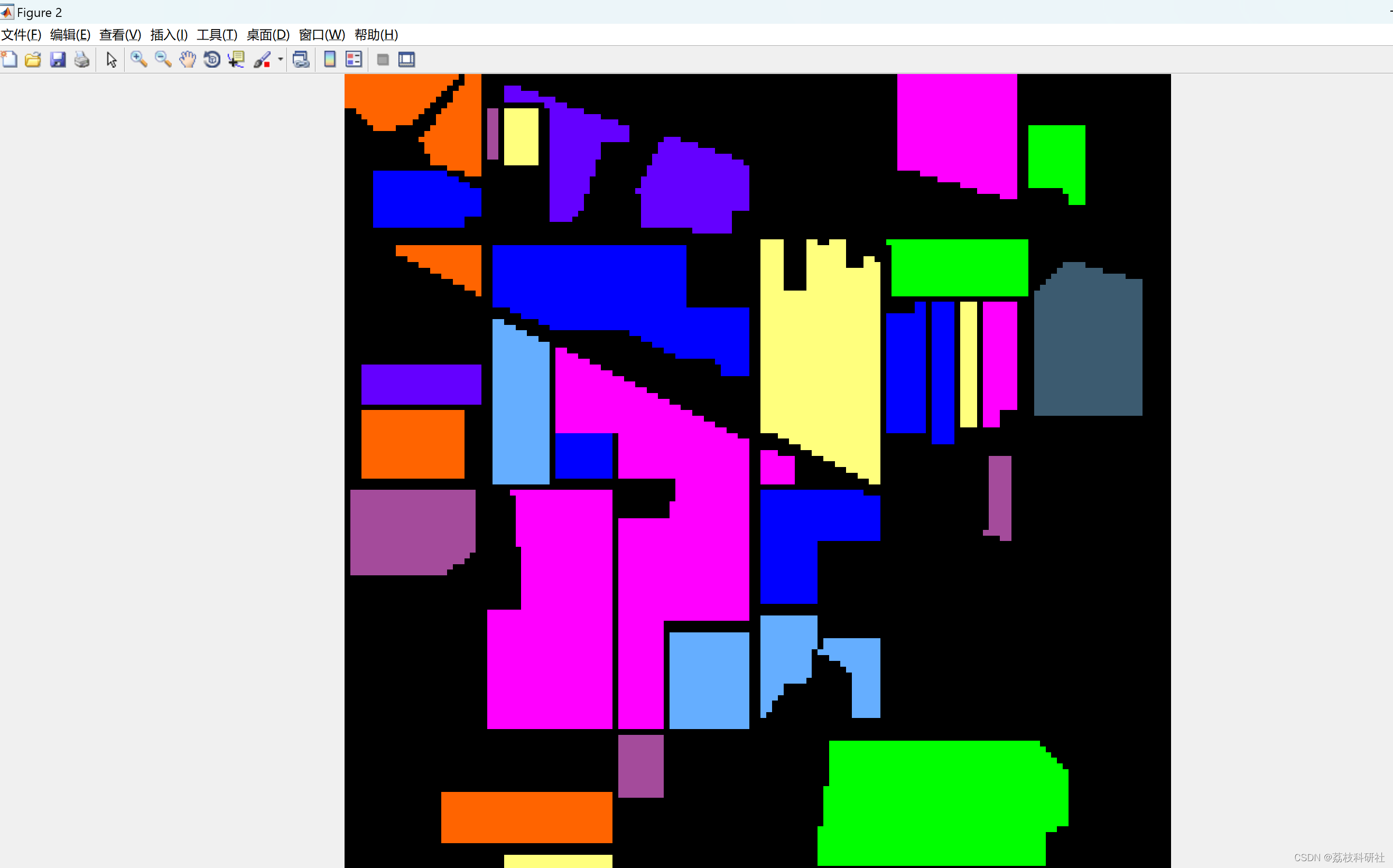
 摘要：我们提出了一种基于稀疏性的轻量级算法，即用于高光谱图像（HSI）分类的基本阈值分类器（BTC）。BTC是一个像素分类器，仅使用给定测试像素的光谱特征。它使用由标记的训练像素组成的预定字典执行分类。然后，它生成测试像素的类标签和残差矢量。由于在HSI分类中纳入空间和光谱信息是提高分类准确性的有效方法，因此我们将建议扩展到三步空间光谱框架。首先，给定HSI的每个像素都使用BTC进行分类。由此产生的残差向量形成一个立方体，可以解释为表示残差图的图像堆栈。其次，使用平均过滤器过滤每个残差图。最后，根据最小残差确定每个测试像素的类标签。在公共数据集上的数值结果表明，我们的提案在分类精度和计算成本方面都优于众所周知的基于支持向量机的技术和基于稀疏的贪婪方法，如同步正交匹配追踪。

原文摘要：

ABSTRACT: We propose a lightweight sparsity-based algorithm, namely, the basic thresholding classifier (BTC), for hyperspectral image (HSI) classification. BTC is a pixelwise classifier which uses only the spectral features of a given test pixel. It performs the classification using a predetermined dictionary consisting of labeled training pixels. It then produces the class label and residual vector of the test pixel. Since incorporating spatial and spectral information in HSI classification is quite an effective way of improving classification accuracy, we extend our proposal to a three-step spatial–spectral framework. First, every pixel of a given HSI is classified using BTC. The resulting residual vectors form a cube which could be interpreted as a stack of images representing residual maps. Second, each residual map is filtered using an averaging filter. Finally, the class label of each test pixel is determined based on minimal residual. Numerical results on public data sets show that our proposal outperforms well-known support vector machine-based techniques and sparsity-based greedy approaches like simultaneous orthogonal matching pursuit in terms of both classification accuracy and computational cost.

地球表面的不同物质具有不同的电磁光谱特征。在给定的 场景中，这些特征可以被具有小空间和光谱分辨率的远程传感器捕获。每个像素 捕获的高光谱图像（HSI）或数据立方体包含非常有用的光谱测量值或特征，这些测量值或特征可能是 用于区分不同的材料和物体。随着传感器技术的进步，电流传感器 能够捕获数百个光谱测量值。但是，增加HSI像素的光谱特征数量 并不总是有助于提高像素的正确分类率。例如，在监督 分类技术，在某些时候，进一步增加输入特征向量的大小可能会减少 分类准确性。这被称为高维问题或休斯现象[1]。

已经提出了几种降维技术来消除休斯现象的影响[2]-[4]。此外，为了提高分类准确性，各种方法都有 被提议。其中，支持向量机（SVM）技术优于经典方法，如K-near。 邻居 （K-NN） 和径向基函数 （RBF） 网络 [5]。已经表明，SVM 在分类方面与众不同 准确性，计算成本和对休斯现象的低脆弱性，并且需要一些训练样本[5]，[6]。另一方面，SVM 方法有一些局限性。首先，它有 参数调整 （C,γ和容错）和内核（线性、RBF 等） 使用 k 折叠交叉验证完成的选择步骤，其中部分训练数据用于 测试目的。这些程序很麻烦，并且生成的参数集可能不是测试集的最佳参数集[7]。其次，由于 SVM 是一个二元分类器，因此将策略转换为 需要多类大小写。一个简单的方法是一对多（OAA）策略，其中测试样本可能导致 未分类，导致分类精度低[7]。另一种策略是一对一（OAO）方法，其中数字 二元分类器(K(K−1）/2)随着类数的增多而急剧增加(K)增加。最后的限制是概率 不能直接提供 SVM 分类器的输出，需要估计程序，例如 logistic 乙状结肠 [8]。因此，使用概率输出的基于 SVM 的方法必须依赖于 这些估计。

前面描述的 SVM 方法属于像素算法类，因为它仅使用光谱特征。 众所周知，像素级分类器的性能可以通过合并空间信息来提高 基于HSI均匀区域中的相邻像素具有相似的光谱特征的事实。 因此，已经提出了各种方法来结合光谱和空间信息。例如，一个 [9] 中提出了复合核方法，该方法成功地提高了 SVM 的分类精度。一个 [10]中提出的基于分割的技术结合了通过聚类和像素获得的分割图 SVM 技术的分类结果。最终决定由自适应定义的多数票做出 窗户。[11]中提出了一个类似的框架，该框架利用分割图使用流域变换。都 这些方法具有共同的局限性，因为它们基于 SVM 方法。

最近的空间光谱框架之一，它利用边缘保持滤波器，已经在[12]中提出。该方法使用 SVM 分类器作为像素分类步骤。 对于每个类，概率图（即 SVM 分类器的后验概率输出）将被平滑处理 通过带有灰度或RGB引导图像的边缘保留滤镜。然后根据每个像素做出最终决定 在最大概率上。作为边缘保护过滤器，它们使用最新的先进技术之一， 即引导图像过滤[13]。由于所提出的框架基于 SVM，因此它也具有通用性 基于 SVM 的分类器的问题。SVM 分类器的一种替代方法是多项式逻辑回归 （国土资源局）[14] 学习类后验概率分布的方法 使用贝叶斯框架。MLR已成功应用于[15]-[17]中的HSI分类。[18]中提出了一种基于MLR的最新技术。该方法通过拆分和增强使用逻辑回归 拉格朗日（LORSAL）[19]算法与主动学习，以估计后验 分布。在分割阶段，它在对空间进行编码之前利用多级逻辑 （MLL） 信息。与传统的分割方法相比，LORSAL-MLL（L-MLL）技术取得了有希望的结果。

 部分代码：

clc; clear all; close all;

addpath('./Dataset') addpath('./KBTC')

% ---- options ------

findGamma = 0; % set to 1 for finding best gamma findThreshold = 0; %set to 1 for finding the best threshold

%trainGroups = 1;% fixed 1 group, %trainGroups = 2;% fixed 2 groups, trainGroups = 3;% fixed 3 groups

alpha = 1e-10; %small alpha in order to prevent ill-condioned matrix inverse

imageName = 'IndianPines'; %imageName = 'Salinas'; %imageName = 'PaviaUni'; %imageName = 'KSC'; %imageName = 'Botswana'; %imageName = 'SalinasA';

%------- dataset options ------- if strcmp(imageName,'IndianPines') == 1          trainPercent = 10;          gamma = 2^-6; M = 95;          delta = 3;        points1 = [28 39; 18 10; 9 78; 29 54; 131 37; 83 47; 37 90; 10 52; 98 125];     points2 =[96 48; 9 63; 49 119; 63 99; 125 47; 29 12; 59 82; 39 9; 105 32];     points3 = [79 80; 28 128; 114 70; 77 98; 130 53; 31 138; 104 7; 57 18; 122 11]; end if strcmp(imageName,'Salinas') == 1          trainPercent = 5;      gamma = 2^-6; M = 92;          delta = 4;   points1 = [9 268; 116 216; 159 164; 87 61; 103 59; 125 45; 154 31; 50 161;         50 419; 18 358; 9 295; 19 306; 22 324; 23 335; 23 70; 9 472];     points2 = [44 246; 147 214; 183 180; 118 123; 131 118; 153 105; 180 85; 94 143;         77 456; 84 319; 42 273; 71 274; 57 304; 72 308; 48 55; 15 498]; end if strcmp(imageName,'PaviaUni') == 1          trainPercent = 5;     gamma = 2^-1; M = 35;          delta = 3;

     points1 = [108 29; 41 114; 34 363; 147 28; 126 168; 188 275; 117 323;         53 163; 93 433];     points2 = [185 173; 90 196; 3 451; 286 341; 161 245; 187 338; 138 365;         82 265; 34 393];     points3 = [331 376; 210 580; 66 386; 167 85; 151 227; 215 329; 142 314;         16 162; 15 436];      end

img = importdata([imageName,'.mat']);

GroundT = importdata([imageName,'_groundT.mat']); no_classes = max(GroundT(:,2));

%discard some classes because of lack of the samples if strcmp(imageName,'IndianPines') == 1     GroundT(GroundT(:,2)==1,:)=[];     GroundT(GroundT(:,2)==7,:)=[];     GroundT(GroundT(:,2)==9,:)=[];     GroundT(GroundT(:,2)==16,:)=[];     GroundT(GroundT(:,2)==4,:)=[];     GroundT(GroundT(:,2)==13,:)=[];     GroundT(GroundT(:,2)==15,:)=[]; end

%%%% estimate the size of the input image [no_lines, no_rows, no_bands] = size(img);

%%%% vectorization img = ToVector(img); img = img';

GroundT=GroundT';

%%%% construct training and test datasets

if trainGroups == 1     indexes = generateFixedIndexes1(no_rows, no_lines, delta, points1, GroundT); elseif trainGroups == 2     indexes = generateFixedIndexes2(no_rows, no_lines, delta, points1, points2, GroundT); elseif trainGroups == 3     indexes = generateFixedIndexes3(no_rows, no_lines, delta, points1, points2, points3, GroundT); end

%%% get the training-test indexes trainIndexes = GroundT(1,indexes); trainLabels = GroundT(2,indexes); groundIndexes = GroundT(1,:); groundLabels = GroundT(2,:); testIndexes = groundIndexes; testLabels = groundLabels; testIndexes(indexes) = []; testLabels(indexes) = [];

%%% get the training-test samples

部分理论来源于网络，如有侵权请联系删除。

[1] M. A. Toksoz and I. Ulusoy, “Hyperspectral Image Classification via Kernel Basic Thresholding Classifier”, IEEE Transactions on Geoscience and Remote Sensing, accepted for publication, 2016. [2] M. A. Toksoz and I. Ulusoy, “Hyperspectral image classification via basic thresholding classifier,” IEEE Transactions on Geoscience and Remote Sensing, vol. 54, no. 7, pp. 4039–4051, 2016. [3] M. A. Toksoz and I. Ulusoy, “Classification via ensembles of basic thresholding classifiers,” IET Computer Vision, 2016, doi:10.1049/ietcvi.2015.0077.