| 机器学习 | 您所在的位置:网站首页 › 编程参数方程是什么 › 机器学习 |
机器学习
|
一、正规方程的引入
当我们求解线性回归问题时引入梯度下降算法的目的是,为了找到代价函数的最小值,也就是代价函数曲线的最低点,如图: 线性回归模型的代价函数为误差平方和代价函数,如下 梯度下降对参数θ求偏导得出: 1、方法一 当代价函数对参数θ求的偏导(上边梯度下降)等于0时,如下: 1、只要特征变量的数目并不大,标准方程是一个很好的计算参数θ的替代方法。 2、只要特征变量数量小于一万,我通常使用标准方程法,而不使用梯度下降法。 3、当讲到分类算法,像逻辑回归算法,我们会看到,实际上对于那些算法,并不能使用标准方程法。 4、对于那些更复杂的学习算法,我们将不得不仍然使用梯度下降法。因此,梯度下降法是一个非常有用的算法。 5、对于那些不可逆的矩阵(通常是因为特征之间不独立,如同时包含英尺为单位的尺寸和米为单位的尺寸两个特征,也有可能是特征数量大于训练集的数量),正规方程方法是不能用的。 四、梯度下降与正规方程的比较
1、 #导库 import numpy as np import matplotlib.pyplot as plt plt.rcParams['font.sans-serif'] = ['SimHei'] #显示中文 plt.rcParams['axes.unicode_minus'] = False #显示负号 #数据集 X=[1.5,0.8,2.6,1.0,0.6,2.8,1.2,0.9,0.4,1.3,1.2,2.0,1.6,1.8,2.2] y=[3.1,1.9,4.2,2.3,1.6,4.9,2.8,2.1,1.4,2.4,2.4,3.8,3.0,3.4,4.0] #数据初始化 X = np.c_[np.ones(len(X)),X] y = np.c_[y] #初始化θ theta = np.zeros((2,1)) #正规方程的代码表示 !!!!重点!!!! theta = np.linalg.inv(X.T.dot(X)).dot(X.T.dot(y)) #可视化展示 画图 plt.figure('散点图') plt.title('散点图') plt.scatter(X[:,1],y,c='r',marker='*',label='样本点') plt.xlabel('X') plt.ylabel('y') theta0 = theta[0] theta1 = theta[1] #画回归方程 min_x,max_x = np.min(X),np.max(X) min_y = theta1*min_x + theta0 max_y = theta1*max_x + theta0 plt.plot((min_x,max_x),(min_y,max_y),c='g') plt.legend() plt.show()结果展示 结果展示 Date Time ... Sub_metering_2 Sub_metering_3 0 16/12/2006 17:24:00 ... 1.0 17.0 1 16/12/2006 17:25:00 ... 1.0 16.0 2 16/12/2006 17:26:00 ... 2.0 17.0 3 16/12/2006 17:27:00 ... 1.0 17.0 4 16/12/2006 17:28:00 ... 1.0 17.0 .. ... ... ... ... ... 995 17/12/2006 09:59:00 ... 0.0 0.0 996 17/12/2006 10:00:00 ... 0.0 0.0 997 17/12/2006 10:01:00 ... 0.0 0.0 998 17/12/2006 10:02:00 ... 0.0 0.0 999 17/12/2006 10:03:00 ... 0.0 18.0 [1000 rows x 9 columns] Int64Index: 999 entries, 1 to 999 Data columns (total 4 columns): Global_active_power 999 non-null object Global_reactive_power 999 non-null float64 Global_intensity 999 non-null float64 b 999 non-null int64 dtypes: float64(2), int64(1), object(1) memory usage: 39.0+ KB None [[4.10551185] [0.68820978] [0.35884791]] |
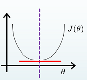 那么当对于某些线性回归问题,我们可不可以直接让代价函数对参数θ求的偏导等于0,来算出代价函数最小时的参数呢?这就引出了正规方程。
 如若对线性回归的算法的推导不是很清晰,可点击下面链接进行学习。 单变量线性回归算法推导及代码实现
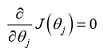 则
则 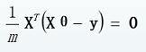 进一步推导出
 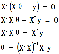 这就是正规方程的最终表达式。 2、方法二

 2、Pandas库
【本文地址】
公司简介
联系我们