| 机器学习笔记之狄利克雷过程(六)预测任务求解 | 您所在的位置:网站首页 › 狄利克雷函数的测度计算 › 机器学习笔记之狄利克雷过程(六)预测任务求解 |
机器学习笔记之狄利克雷过程(六)预测任务求解
|
机器学习笔记之狄利克雷过程——预测任务求解
引言回顾:基于狄利克雷过程的预测过程预测任务的求解过程
引言
上一节引出了基于狄利克雷过程的预测任务,本节将对该预测任务进行求解。 回顾:基于狄利克雷过程的预测过程在已知隐变量样本集合 θ = { θ ( i ) } i = 1 N \theta = \{\theta^{(i)}\}_{i=1}^N θ={θ(i)}i=1N的条件下,关于一个陌生样本 θ ^ \hat {\theta} θ^的后验概率分布 P ( θ ^ ∣ θ ) \mathcal P(\hat \theta \mid \theta) P(θ^∣θ)可表示为: P ( θ ^ ∣ θ ) = ∑ G P ( θ ^ ∣ G ) ⋅ P ( G ∣ θ ) \mathcal P(\hat \theta \mid \theta) = \sum_{\mathcal G} \mathcal P(\hat \theta \mid \mathcal G) \cdot \mathcal P(\mathcal G \mid \theta) P(θ^∣θ)=G∑P(θ^∣G)⋅P(G∣θ) 其中 P ( G ∣ θ ) \mathcal P(\mathcal G \mid \theta) P(G∣θ)是指随机测度 G \mathcal G G的后验概率分布;而 P ( θ ^ ∣ G ) \mathcal P(\hat \theta \mid \mathcal G) P(θ^∣G)表示关于陌生隐变量样本的预测分布。 这个预测分布最终会得到一个 θ \theta θ具体数值的概率分布。但实际上,我们对预测出的 θ \theta θ数值并不关心,我们更关心的是哪些 θ ( i ) \theta^{(i)} θ(i)样本,它们的 θ \theta θ数值相等。 因为一旦 θ ( i ) = θ ( j ) ( i ≠ j ; θ ( i ) , θ ( j ) ∈ θ ) \theta^{(i)} = \theta^{(j)}(i \neq j;\theta^{(i)},\theta^{(j)} \in \theta) θ(i)=θ(j)(i=j;θ(i),θ(j)∈θ)这就意味着对应的 θ ( i ) ⇒ x ( i ) , θ ( j ) ⇒ x ( j ) \theta^{(i)}\Rightarrow x^{(i)},\theta^{(j)} \Rightarrow x^{(j)} θ(i)⇒x(i),θ(j)⇒x(j)属于同一类别。但 θ ( i ) = θ ( j ) = ? \theta^{(i)} = \theta^{(j)} = ? θ(i)=θ(j)=?这个值我们并不关心。 假设每个真实样本均隐含地存在一个聚类标签: Z = { z ( i ) } i = 1 N \mathcal Z = \{z^{(i)}\}_{i=1}^N Z={z(i)}i=1N,那么最终的将预测过程转化为: P ( z ^ ∣ Z ) \mathcal P(\hat z \mid \mathcal Z) P(z^∣Z)。 关于真实样本 x ^ \hat x x^最终被划分到了哪个具体类别——才是真正关心的信息,而 Z \mathcal Z Z则表示数据集合中样本点对应的标签结果。 预测任务的求解过程关于预测任务的转化结果表达如下: P ( z ^ = m ∣ Z ) Z = { z ( 1 ) , z ( 2 ) , ⋯ , z ( N ) } \mathcal P(\hat z = m \mid \mathcal Z) \quad \mathcal Z = \{z^{(1)},z^{(2)},\cdots,z^{(N)}\} P(z^=m∣Z)Z={z(1),z(2),⋯,z(N)} 其中 z ^ \hat z z^是对应陌生样本的隐含标签;而 m m m则表示这个离散标签可选择的某个结果。首先,通过贝叶斯定理,可以将上式表示为如下形式: P ( z ^ = m ∣ Z ) = P ( z ^ = m , Z ) P ( Z ) \mathcal P(\hat z = m \mid \mathcal Z) = \frac{\mathcal P(\hat z = m,\mathcal Z)}{\mathcal P(\mathcal Z)} P(z^=m∣Z)=P(Z)P(z^=m,Z) 其次将狄利克雷过程引入进来。但由于狄利克雷过程中可能包含无穷多个随机变量 θ 1 , θ 2 , ⋯ , θ ∞ \theta_1,\theta_2,\cdots,\theta_{\infty} θ1,θ2,⋯,θ∞(它的随机变量数量由 α \alpha α决定)。关于对狄利克雷过程中随机变量的积分是复杂的。这里退而求其次,首先引入一个狄利克雷分布: P ( G ) = DP ( α , H ) = P [ G ( a 1 ) , G ( a 2 ) , ⋯ , G ( a D ) ] \mathcal P(\mathcal G) = \text{DP}(\alpha,\mathcal H)= \mathcal P[\mathcal G(a_1),\mathcal G(a_2),\cdots,\mathcal G(a_{\mathcal D})] P(G)=DP(α,H)=P[G(a1),G(a2),⋯,G(aD)] 上式 P ( G ) \mathcal P(\mathcal G) P(G)明显是随机测度 G \mathcal G G的先验分布,而随机测度 G \mathcal G G就是通过狄利克雷过程 DP ( α , H ) \text{DP}(\alpha,\mathcal H) DP(α,H)生成的,因而 P ( G ) = DP ( α , H ) \mathcal P(\mathcal G) = \text{DP}(\alpha,\mathcal H) P(G)=DP(α,H); G ( a 1 ) , ⋯ , G ( a D ) \mathcal G(a_1),\cdots,\mathcal G(a_{\mathcal D}) G(a1),⋯,G(aD)分别表示随机测度 G \mathcal G G的的样本空间被划分成 D \mathcal D D个区域,各个区域原子数量的结果。根据狄利克雷过程的核心性质,可以将上式转化为: P [ G ( a 1 ) , G ( a 2 ) , ⋯ , G ( a D ) ] = Dir [ α H ( a 1 ) , α H ( a 2 ) , ⋯ , α H ( a D ) ] \mathcal P[\mathcal G(a_1),\mathcal G(a_2),\cdots,\mathcal G(a_{\mathcal D})] = \text{Dir}[\alpha \mathcal H(a_1),\alpha \mathcal H(a_2),\cdots,\alpha \mathcal H(a_{\mathcal D})] P[G(a1),G(a2),⋯,G(aD)]=Dir[αH(a1),αH(a2),⋯,αH(aD)] 这里不妨设基本测度 H \mathcal H H是一个均匀分布,则有: { H ( a 1 ) = H ( a 2 ) = ⋯ = H ( a D ) = 1 D ∑ d = 1 D H ( a d ) = 1 Dir [ α H ( a 1 ) , α H ( a 2 ) , ⋯ , α H ( a D ) ] = Dir ( α D , α D , ⋯ , α D ⏟ D 个 ) \begin{cases} \mathcal H(a_1) = \mathcal H(a_2)= \cdots = \mathcal H(a_{\mathcal D}) = \frac{1}{\mathcal D} \quad \sum_{d=1}^{\mathcal D} \mathcal H(a_d) = 1 \\ \text{Dir}[\alpha \mathcal H(a_1),\alpha \mathcal H(a_2),\cdots,\alpha \mathcal H(a_{\mathcal D})] = \text{Dir} \left(\underbrace{\frac{\alpha}{\mathcal D},\frac{\alpha}{\mathcal D},\cdots,\frac{\alpha}{\mathcal D}}_{\mathcal D个}\right) \end{cases} ⎩ ⎨ ⎧H(a1)=H(a2)=⋯=H(aD)=D1∑d=1DH(ad)=1Dir[αH(a1),αH(a2),⋯,αH(aD)]=Dir D个 Dα,Dα,⋯,Dα 至此,将狄利克雷分布引入到 P ( z ^ = m ∣ Z ) \mathcal P(\hat z = m \mid \mathcal Z) P(z^=m∣Z)中: P ( z ^ = m ∣ Z ) = P ( z ^ = m , Z ) P ( Z ) = ∑ G ( a 1 ) , ⋯ , ∑ G ( a D ) P [ z ^ = m , Z ∣ G ( a 1 ) , ⋯ , G ( a D ) ] ⋅ P [ G ( a 1 ) , ⋯ , G ( a D ) ] ∑ G ( a 1 ) , ⋯ , ∑ G ( a D ) P [ Z ∣ G ( a 1 ) , ⋯ , G ( a D ) ] ⋅ P [ G ( a 1 ) , ⋯ , G ( a D ) ] \begin{aligned} \mathcal P(\hat z = m \mid \mathcal Z) & = \frac{\mathcal P(\hat z = m,\mathcal Z)}{\mathcal P(\mathcal Z)} \\ & = \frac{\sum_{\mathcal G(a_1)},\cdots,\sum_{\mathcal G(a_{\mathcal D})} \mathcal P[\hat z = m,\mathcal Z \mid \mathcal G(a_1),\cdots, \mathcal G(a_{\mathcal D})] \cdot \mathcal P[\mathcal G(a_1),\cdots,\mathcal G(a_{\mathcal D})]}{\sum_{\mathcal G(a_1)},\cdots,\sum_{\mathcal G(a_{\mathcal D})} \mathcal P[\mathcal Z \mid \mathcal G(a_1),\cdots,\mathcal G(a_{\mathcal D})] \cdot \mathcal P[\mathcal G(a_1),\cdots,\mathcal G(a_{\mathcal D})]} \\ \end{aligned} P(z^=m∣Z)=P(Z)P(z^=m,Z)=∑G(a1),⋯,∑G(aD)P[Z∣G(a1),⋯,G(aD)]⋅P[G(a1),⋯,G(aD)]∑G(a1),⋯,∑G(aD)P[z^=m,Z∣G(a1),⋯,G(aD)]⋅P[G(a1),⋯,G(aD)] 再将狄利克雷分布代入,有: P ( z ^ = m ∣ Z ) = ∑ G ( a 1 ) , ⋯ , ∑ G ( a D ) P [ z ^ = m , Z ∣ G ( a 1 ) , ⋯ , G ( a D ) ] ⋅ Dir ( α D , α D , ⋯ , α D ) ∑ G ( a 1 ) , ⋯ , ∑ G ( a D ) P [ Z ∣ G ( a 1 ) , ⋯ , G ( a D ) ] ⋅ Dir ( α D , α D , ⋯ , α D ) \mathcal P(\hat z = m \mid \mathcal Z) = \frac{\sum_{\mathcal G(a_1)},\cdots,\sum_{\mathcal G(a_{\mathcal D})} \mathcal P[\hat z = m,\mathcal Z \mid \mathcal G(a_1),\cdots,\mathcal G(a_{\mathcal D})] \cdot \text{Dir}\left(\frac{\alpha}{\mathcal D},\frac{\alpha}{\mathcal D},\cdots,\frac{\alpha}{\mathcal D}\right)}{\sum_{\mathcal G(a_1)},\cdots,\sum_{\mathcal G(a_{\mathcal D})} \mathcal P[\mathcal Z \mid \mathcal G(a_1),\cdots,\mathcal G(a_{\mathcal D})] \cdot \text{Dir}\left(\frac{\alpha}{\mathcal D},\frac{\alpha}{\mathcal D},\cdots,\frac{\alpha}{\mathcal D}\right)} P(z^=m∣Z)=∑G(a1),⋯,∑G(aD)P[Z∣G(a1),⋯,G(aD)]⋅Dir(Dα,Dα,⋯,Dα)∑G(a1),⋯,∑G(aD)P[z^=m,Z∣G(a1),⋯,G(aD)]⋅Dir(Dα,Dα,⋯,Dα) 通过观察,分子分母非常相似,先从求解分子开始: ∑ G ( a 1 ) , ⋯ , ∑ G ( a D ) P [ z ^ = m , Z ∣ G ( a 1 ) , ⋯ , G ( a D ) ] ⋅ Dir ( α D , α D , ⋯ , α D ) \sum_{\mathcal G(a_1)},\cdots,\sum_{\mathcal G(a_{\mathcal D})} \mathcal P[\hat z = m,\mathcal Z \mid \mathcal G(a_1),\cdots,\mathcal G(a_{\mathcal D})] \cdot \text{Dir}\left(\frac{\alpha}{\mathcal D},\frac{\alpha}{\mathcal D},\cdots,\frac{\alpha}{\mathcal D}\right) G(a1)∑,⋯,G(aD)∑P[z^=m,Z∣G(a1),⋯,G(aD)]⋅Dir(Dα,Dα,⋯,Dα) 其中 P [ z ^ = m , Z ∣ G ( a 1 ) , ⋯ , G ( a D ) ] \mathcal P[\hat z = m,\mathcal Z \mid \mathcal G(a_1),\cdots,\mathcal G(a_{\mathcal D})] P[z^=m,Z∣G(a1),⋯,G(aD)]表示关于 z ^ , Z \hat z,\mathcal Z z^,Z的似然分布,是一个多项式分布。根据指数族分布的共轭性质,积分内的乘积结果同样是狄利克雷分布。将积分号内各项的概率密度函数表示出来: 该项本质上是关于后验分布的推导过程 分子用符号 I n u m e r \mathcal I_{numer} Inumer表示。其中 z ^ , Z \hat z,\mathcal Z z^,Z表示聚类标签的具体分布,并且它们的分布与随机测度 G \mathcal G G的离散数量相同。假设 z ^ , Z \hat z,\mathcal Z z^,Z的离散随机变量是 z 1 , ⋯ , z D z_1,\cdots,z_{\mathcal D} z1,⋯,zD. I n u m e r = ∑ G ( a 1 ) , ⋯ , ∑ G ( a D ) ( ( ∑ d = 1 D z d ) ! z 1 ! ⋯ z D ! ∏ d = 1 D G ( a d ) z d ) ⋅ ( Γ [ α ∑ d = 1 D 1 D ] ∏ d = 1 D Γ ( α ∑ d = 1 D 1 D ) ∏ d = 1 D G ( a d ) α D − 1 ) \mathcal I_{numer} = \sum_{\mathcal G(a_1)},\cdots,\sum_{\mathcal G(a_{\mathcal D})} \left(\frac{\left(\sum_{d=1}^{\mathcal D} z_d\right)!}{z_1! \cdots z_{\mathcal D}!} \prod_{d=1}^{\mathcal D} \mathcal G(a_d)^{z_d}\right) \cdot \left(\frac{\Gamma \left[\alpha\sum_{d=1}^{\mathcal D} \frac{1}{\mathcal D}\right]}{\prod_{d=1}^{\mathcal D}\Gamma(\alpha\sum_{d=1}^{\mathcal D} \frac{1}{\mathcal D})}\prod_{d=1}^{\mathcal D}\mathcal G(a_d)^{\frac{\alpha}{\mathcal D} - 1}\right) Inumer=G(a1)∑,⋯,G(aD)∑ z1!⋯zD!(∑d=1Dzd)!d=1∏DG(ad)zd ⋅ ∏d=1DΓ(α∑d=1DD1)Γ[α∑d=1DD1]d=1∏DG(ad)Dα−1 从概率密度积分的角度观察: 由于多项式分布是狄利克雷分布的共轭先验,根据贝叶斯定理,分子积分内的项必然与狄利克雷分布之间存在常数的系数关系: 这里假设这个常数项是 C = P ( z ^ , Z ) \mathcal C = \mathcal P(\hat z,\mathcal Z) C=P(z^,Z),对应的后验狄利克雷分布记作 Dir p o s t \text{Dir}_{post} Dirpost. C ⋅ Dir p o s t = P [ z ^ = m , Z ∣ G ( a 1 ) , ⋯ , G ( a D ) ] ⋅ Dir ( α D , α D , ⋯ , α D ) ⇒ Dir p o s t ∝ P [ z ^ = m , Z ∣ G ( a 1 ) , ⋯ , G ( a D ) ] ⋅ Dir ( α D , α D , ⋯ , α D ) ⇒ I n u m e r = ∑ G ( a 1 ) , ⋯ , ∑ G ( a D ) C ⋅ Dir p o s t ∝ ∑ G ( a 1 ) , ⋯ , ∑ G ( a D ) Dir p o s t \begin{aligned} & \mathcal C \cdot \text{Dir}_{post} = \mathcal P[\hat z = m,\mathcal Z \mid \mathcal G(a_1),\cdots,\mathcal G(a_{\mathcal D})] \cdot \text{Dir}\left(\frac{\alpha}{\mathcal D},\frac{\alpha}{\mathcal D},\cdots,\frac{\alpha}{\mathcal D}\right) \\ & \Rightarrow \text{Dir}_{post} \propto \mathcal P[\hat z = m,\mathcal Z \mid \mathcal G(a_1),\cdots,\mathcal G(a_{\mathcal D})] \cdot \text{Dir}\left(\frac{\alpha}{\mathcal D},\frac{\alpha}{\mathcal D},\cdots,\frac{\alpha}{\mathcal D}\right) \\ & \Rightarrow \mathcal I_{numer} = \sum_{\mathcal G(a_1)},\cdots,\sum_{\mathcal G(a_{\mathcal D})} \mathcal C \cdot \text{Dir}_{post} \propto \sum_{\mathcal G(a_1)},\cdots,\sum_{\mathcal G(a_{\mathcal D})} \text{Dir}_{post} \end{aligned} C⋅Dirpost=P[z^=m,Z∣G(a1),⋯,G(aD)]⋅Dir(Dα,Dα,⋯,Dα)⇒Dirpost∝P[z^=m,Z∣G(a1),⋯,G(aD)]⋅Dir(Dα,Dα,⋯,Dα)⇒Inumer=G(a1)∑,⋯,G(aD)∑C⋅Dirpost∝G(a1)∑,⋯,G(aD)∑Dirpost针对上式第二步, ∝ \propto ∝左右两侧的概率分布分别对各自的随机变量进行积分: 1 = ∑ G ( a 1 ) , ⋯ , ∑ G ( a D ) Dir p o s t ∝ ∑ G ( a 1 ) , ⋯ , ∑ G ( a D ) ( ( ∑ d = 1 D z d ) ! z 1 ! ⋯ z D ! ∏ d = 1 D G ( a d ) z d ) ⋅ ( Γ [ α ∑ d = 1 D 1 D ] ∏ d = 1 D Γ ( α ∑ d = 1 D 1 D ) ∏ d = 1 D G ( a d ) α D − 1 ) = { ( ∑ d = 1 D z d ) ! z 1 ! ⋯ z D ! ⋅ Γ [ α ∑ d = 1 D 1 D ] ∏ d = 1 D Γ ( α ∑ d = 1 D 1 D ) } ⏟ 前项 ⋅ ∑ G ( a 1 ) , ⋯ , ∑ G ( a D ) [ ∏ d = 1 D G ( a d ) z d + α D − 1 ] ⏟ 后项 \begin{aligned} 1 = \sum_{\mathcal G(a_1)},\cdots,\sum_{\mathcal G(a_{\mathcal D})} \text{Dir}_{post} & \propto \sum_{\mathcal G(a_1)},\cdots,\sum_{\mathcal G(a_{\mathcal D})} \left(\frac{\left(\sum_{d=1}^{\mathcal D} z_d\right)!}{z_1! \cdots z_{\mathcal D}!} \prod_{d=1}^{\mathcal D} \mathcal G(a_d)^{z_d}\right) \cdot \left(\frac{\Gamma \left[\alpha\sum_{d=1}^{\mathcal D} \frac{1}{\mathcal D}\right]}{\prod_{d=1}^{\mathcal D}\Gamma(\alpha\sum_{d=1}^{\mathcal D} \frac{1}{\mathcal D})}\prod_{d=1}^{\mathcal D}\mathcal G(a_d)^{\frac{\alpha}{\mathcal D} - 1}\right) \\ & = \underbrace{\left\{\frac{\left(\sum_{d=1}^{\mathcal D} z_d\right)!}{z_1! \cdots z_{\mathcal D}!} \cdot \frac{\Gamma \left[\alpha\sum_{d=1}^{\mathcal D} \frac{1}{\mathcal D}\right]}{\prod_{d=1}^{\mathcal D}\Gamma(\alpha\sum_{d=1}^{\mathcal D} \frac{1}{\mathcal D})}\right\}}_{前项} \cdot \underbrace{\sum_{\mathcal G(a_1)},\cdots,\sum_{\mathcal G(a_{\mathcal D})} \left[\prod_{d=1}^{\mathcal D}\mathcal G(a_d)^{z_d + \frac{\alpha}{\mathcal D} - 1}\right]}_{后项} \end{aligned} 1=G(a1)∑,⋯,G(aD)∑Dirpost∝G(a1)∑,⋯,G(aD)∑ z1!⋯zD!(∑d=1Dzd)!d=1∏DG(ad)zd ⋅ ∏d=1DΓ(α∑d=1DD1)Γ[α∑d=1DD1]d=1∏DG(ad)Dα−1 =前项 ⎩ ⎨ ⎧z1!⋯zD!(∑d=1Dzd)!⋅∏d=1DΓ(α∑d=1DD1)Γ[α∑d=1DD1]⎭ ⎬ ⎫⋅后项 G(a1)∑,⋯,G(aD)∑[d=1∏DG(ad)zd+Dα−1] 关于后项 ∑ G ( a 1 ) , ⋯ , ∑ G ( a D ) [ ∏ d = 1 D G ( a d ) z d + α D − 1 ] \sum_{\mathcal G(a_1)},\cdots,\sum_{\mathcal G(a_{\mathcal D})} \left[\prod_{d=1}^{\mathcal D}\mathcal G(a_d)^{z_d + \frac{\alpha}{\mathcal D} - 1}\right] ∑G(a1),⋯,∑G(aD)[∏d=1DG(ad)zd+Dα−1]可以近似地看作前项的倒数: 之所以是近似,是因为 1 1 1和前项X后项之间仅是 ∝ \propto ∝关系,而不是 = = =关系。 Γ \Gamma Γ函数是一个以 exp \exp exp为底的指数函数,将连乘项直接代入到 Γ \Gamma Γ函数中。并且 ∑ d = 1 D 1 D = 1 \sum_{d=1}^{\mathcal D} \frac{1}{\mathcal D} = 1 ∑d=1DD1=1直接消掉了。 ∑ d = 1 D \sum_{d=1}^{\mathcal D} ∑d=1D本身就表示多项式分布的随机变量集合,这里直接使用 Z \mathcal Z Z进行表示。 ∑ G ( a 1 ) , ⋯ , ∑ G ( a D ) [ ∏ d = 1 D G ( a d ) z d + α D − 1 ] ∝ z 1 ! ⋯ z D ! ( ∑ d = 1 D z d ) ! ⋅ ∏ d = 1 D Γ ( α ∑ d = 1 D 1 D ) Γ [ α ∑ d = 1 D 1 D ] = ∏ d = 1 D Γ ( α + z d ) Γ [ α + Z ] \begin{aligned} \sum_{\mathcal G(a_1)},\cdots,\sum_{\mathcal G(a_{\mathcal D})} \left[\prod_{d=1}^{\mathcal D}\mathcal G(a_d)^{z_d + \frac{\alpha}{\mathcal D} - 1}\right] & \propto \frac{z_1 !\cdots z_{\mathcal D}!}{\left(\sum_{d=1}^{\mathcal D} z_d\right)!} \cdot \frac{\prod_{d=1}^{\mathcal D} \Gamma \left(\alpha \sum_{d=1}^{\mathcal D} \frac{1}{\mathcal D}\right)}{\Gamma \left[\alpha \sum_{d=1}^{\mathcal D} \frac{1}{\mathcal D}\right]} \\ & = \frac{\prod_{d=1}^{\mathcal D} \Gamma \left(\alpha + z_d\right)}{\Gamma \left[\alpha + \mathcal Z\right]} \end{aligned} G(a1)∑,⋯,G(aD)∑[d=1∏DG(ad)zd+Dα−1]∝(∑d=1Dzd)!z1!⋯zD!⋅Γ[α∑d=1DD1]∏d=1DΓ(α∑d=1DD1)=Γ[α+Z]∏d=1DΓ(α+zd)最终整理,可以得到关于分子 I n u m e r \mathcal I_{numer} Inumer表示如下: I n u m e r = { ( ∑ d = 1 D z d ) ! z 1 ! ⋯ z D ! ⋅ Γ [ α ∑ d = 1 D 1 D ] ∏ d = 1 D Γ ( α ∑ d = 1 D 1 D ) } ⋅ ∏ d = 1 D Γ ( α + z d ) Γ [ α + Z ] \mathcal I_{numer} = \left\{\frac{\left(\sum_{d=1}^{\mathcal D} z_d\right)!}{z_1! \cdots z_{\mathcal D}!} \cdot \frac{\Gamma \left[\alpha\sum_{d=1}^{\mathcal D} \frac{1}{\mathcal D}\right]}{\prod_{d=1}^{\mathcal D}\Gamma(\alpha\sum_{d=1}^{\mathcal D} \frac{1}{\mathcal D})}\right\} \cdot \frac{\prod_{d=1}^{\mathcal D} \Gamma \left(\alpha + z_d\right)}{\Gamma \left[\alpha + \mathcal Z\right]} Inumer=⎩ ⎨ ⎧z1!⋯zD!(∑d=1Dzd)!⋅∏d=1DΓ(α∑d=1DD1)Γ[α∑d=1DD1]⎭ ⎬ ⎫⋅Γ[α+Z]∏d=1DΓ(α+zd) 但需要做几点说明: 虽然 ( ∑ d = 1 D z d ) ! z 1 ! ⋯ z D ! \frac{\left(\sum_{d=1}^{\mathcal D} z_d\right)!}{z_1! \cdots z_{\mathcal D}!} z1!⋯zD!(∑d=1Dzd)!描述的是多项式分布的系数,但 z 1 , ⋯ , z D z_1,\cdots,z_{\mathcal D} z1,⋯,zD分别表示统计样本属于各个划分的数量,这种统计方式在聚类任务中是不合理的。 例如某样本分布及对应划分如下图所示: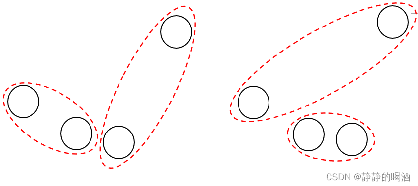 上述2组,每组4个样本分布完全相同,两种划分方式的多项式分布系数均相同,均等于6;但从聚类角度观察,它们是差异极大的两种聚类。因而对
I
n
u
m
e
r
\mathcal I_{numer}
Inumer表示时,删除多项式分布系数的影响。关于狄利克雷分布的系数
Γ
[
α
∑
d
=
1
D
1
D
]
∏
d
=
1
D
Γ
(
α
∑
d
=
1
D
1
D
)
\frac{\Gamma \left[\alpha\sum_{d=1}^{\mathcal D} \frac{1}{\mathcal D}\right]}{\prod_{d=1}^{\mathcal D}\Gamma(\alpha\sum_{d=1}^{\mathcal D} \frac{1}{\mathcal D})}
∏d=1DΓ(α∑d=1DD1)Γ[α∑d=1DD1],无论是分子还是分母,关于先验分布均是从同一个狄利克雷过程中生成的。这意味着划分空间数量
D
\mathcal D
D是固定的。分子分母项可以同时消掉该部分系数。 上述2组,每组4个样本分布完全相同,两种划分方式的多项式分布系数均相同,均等于6;但从聚类角度观察,它们是差异极大的两种聚类。因而对
I
n
u
m
e
r
\mathcal I_{numer}
Inumer表示时,删除多项式分布系数的影响。关于狄利克雷分布的系数
Γ
[
α
∑
d
=
1
D
1
D
]
∏
d
=
1
D
Γ
(
α
∑
d
=
1
D
1
D
)
\frac{\Gamma \left[\alpha\sum_{d=1}^{\mathcal D} \frac{1}{\mathcal D}\right]}{\prod_{d=1}^{\mathcal D}\Gamma(\alpha\sum_{d=1}^{\mathcal D} \frac{1}{\mathcal D})}
∏d=1DΓ(α∑d=1DD1)Γ[α∑d=1DD1],无论是分子还是分母,关于先验分布均是从同一个狄利克雷过程中生成的。这意味着划分空间数量
D
\mathcal D
D是固定的。分子分母项可以同时消掉该部分系数。
最终,可以将分子 I n u m e r \mathcal I_{numer} Inumer表示为: I n u m e r ⇒ ∏ d = 1 D Γ ( α + z d ) Γ [ α + Z ] \mathcal I_{numer} \Rightarrow \frac{\prod_{d=1}^{\mathcal D} \Gamma \left(\alpha + z_d\right)}{\Gamma \left[\alpha + \mathcal Z\right]} Inumer⇒Γ[α+Z]∏d=1DΓ(α+zd) 相关参考: 徐亦达机器学习:Dirichlet-Process-part 7 |
【本文地址】