| 深度学习基础(二) | 您所在的位置:网站首页 › 深度神经网络和卷积神经网络的关系 › 深度学习基础(二) |
深度学习基础(二)
|
经典的多层感知机(Multi-Layer Perceptron)形式上是全连接(fully-connected)的邻接网络(adjacent network)。 That is, every neuron in the network is connected to every neuron in adjacent layers. 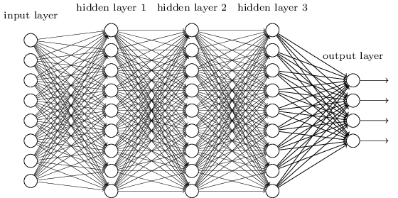 Local receptive fields
全连接的多层感知机中,输入视为(或者需转化为)一个列向量。而在卷积神经网络中,以手写字符识别为例,输入不再 reshape 为 (28*28, 1) 的列向量,而是作为 28×28 的像素灰度矩阵。 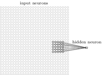
That region in the input image is called the local receptive field for the hidden neuron. It’s a little window on the input pixels. Each connection learns a weight(one single weight,也即整个 5×5 的 region 共享同一个 weight). And the hidden neuron learns an overall bias as well. Shared weights and biases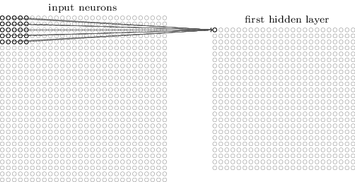 注意对应关系,是左上角对应左上角,后四列是利用不到的?
28×28(5×5)⇒24×24
第
j
行 k 列的隐层神经元的输入为:
b+∑ℓ=04∑m=04wℓ,maj+ℓ,k+m
注意对应关系,是左上角对应左上角,后四列是利用不到的?
28×28(5×5)⇒24×24
第
j
行 k 列的隐层神经元的输入为:
b+∑ℓ=04∑m=04wℓ,maj+ℓ,k+m
该隐层神经元的输出为: σ(b+∑ℓ=04∑m=04wℓ,maj+ℓ,k+m)The network structure I’ve described so far can detect just a single kind of localized feature. To do image recognition we’ll need more than one feature map(特征映射). And so a complete convolutional layer consists of several different feature maps: 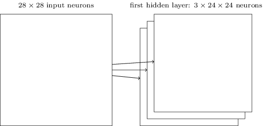
feature map:filter,kernel In the example shown, there are 3 feature maps. Each feature map is defined by a set of 5×5 shared weights, and a single shared bias. The result is that the network can detect 3 different kinds of features(特征检测), with each feature being detectable across the entire image. I’ve shown just 3 feature maps, to keep the diagram above simple. However, in practice convolutional networks may use more (and perhaps many more) feature maps. One of the early convolutional networks, LeNet-5, used 6 feature maps, each associated to a 5×5 local receptive field, to recognize MNIST digits. So the example illustrated above is actually pretty close to LeNet-5. In the examples we develop later in the chapter we’ll use convolutional layers with 20 and 40 feature maps. Let’s take a quick peek at some of the features which are learned* |
【本文地址】