| How to Create Drop Down Lists in Excel | 您所在的位置:网站首页 › 排比修辞的作用和好处 › How to Create Drop Down Lists in Excel |
How to Create Drop Down Lists in Excel
|
Bottom Line: The complete Excel guide on how to create drop-down lists in cells (data validation lists). Includes keyboard shortcuts to select items, copying drop-downs to other cells, handling invalid inputs, updating lists with new items, and more. Skill Level: Beginner Video Tutorial Watch on YouTube & Subscribe to our Channel Download the Excel FileYou can download the file I’m using in the video here: Data-Validation-Lists-Examples.xlsxDownload What Are Data Validation Lists?Creating a drop-down list is a great way to ensure that entries are uniform and free from spelling errors. It also helps restrict entries so that only values you’ve approved make it onto the sheet. That’s why they are also called data validation lists. They help to make sure that only valid data makes it into the cells that you’ve applied it to. 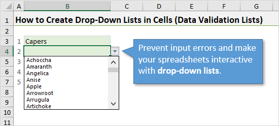
This can be helpful when multiple users are entering data on the same sheet and you want the options to be limited to a list of items or values that you’ve already approved. We can also use drop-down lists to create interactive reports and financial models, where results change when the user changes a cell’s value. How to Create a Drop-down (Data Validation) ListTo create a drop-down list, start by going to the Data tab on the Ribbon and click the Data Validation button. 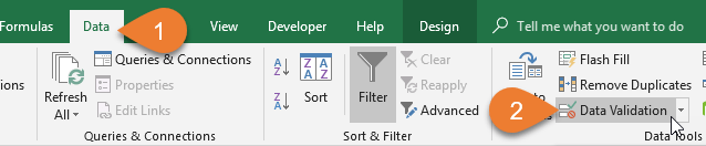
The Data Validation window will appear. The keyboard shortcut to open the Data Validation window is Alt, A, V, V. You’ll want to select List in the drop-down menu under Allow. 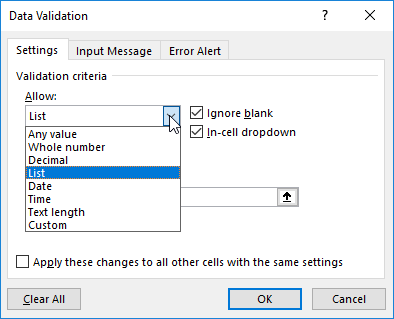
At this point there are a few ways that you can tell Excel what items you want to include in your drop-down list. Drop-down List from Comma Separated ValuesThe first way is by typing all of the options that you want in your drop-down list, separated by commas, into the Source field. For example, if there are only two options to choose from, such as Yes and No, you would simply type “Yes, No” (do not include the quotation marks) in the Source box. It doesn’t matter whether a space follows your comma or not. A longer list of options might look like this: “Red, Blue, Green, Purple, Orange, Yellow, Brown”. The options in your drop-down list will appear in the exact same order that you have typed them. 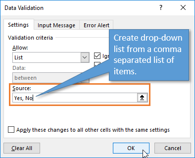
Note: On some language versions of Excel you will need to use a semicolon (;) instead of a comma. Drop-down List from a Range of ValuesThe second way to fill your list with options is to choose them from a range of values. To do this, instead of typing values into the Source field, you want to select the icon to the right. 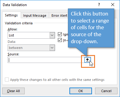
Selecting this icon will open up a small window that will auto-fill when you select a range of cells on the worksheet. Once you've selected the values you want to appear in your drop-down list, you can click on the corresponding icon to take you back to the Data Validation window. 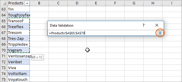
At this point, the range you've selected will show in the Source box and you can just hit OK. 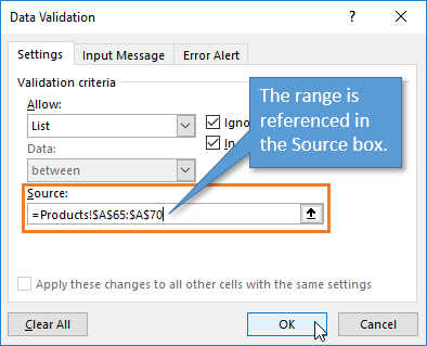
Now the values in the range that you've selected show as options that you can choose from in your drop-down list. 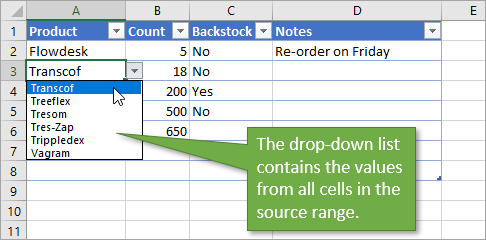 Shortcut for Selecting from the Drop-down List
To choose the option you want from your drop-down list, you can use your mouse to click on the option you want. Another way to select it is to use the keyboard shortcut Alt+?. This brings up the drop-down list and you can use your up and down arrow keys to highlight the selection you want, and then press Enter to select. 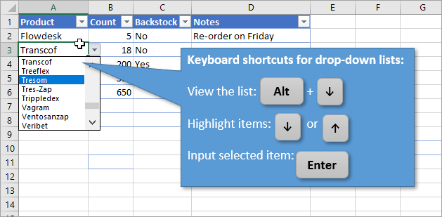 How to Search the Drop-down List
Unfortunately, Excel doesn't have an option to search the drop-down list for a particular item, but I've created an add-in that gives you that option. It's called List Search and you can access that add-in here: 
Click here to download the List Search Add-in Note: You will create a free account for the Excel Campus Members site to access the download and any future updates. The download site also contains installation instructions and videos. How to Copy the Data Validation List to Other CellsIf you have created a drop-down list for a particular cell and would like other cells to have the same data validation list, you can easily copy (extend) that list to other cells. Start by clicking on the cell that has the list, and then select any additional cells that you want to extend the drop-down list to. This can include blank cells or cells that already have values in them. 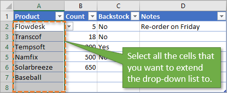
As before, you will click on the Data Validation button in the Data tab, but this time a warning will appear that says, “The selection contains some cells without Data Validation settings. Do you want to extend the Data Validation to these cells?” 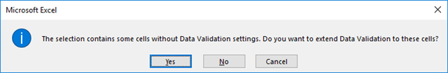
Choose Yes, and then hit OK when the Data Validation Window appears. You'll see that each of the cells in your selection now has the same drop-down options as the original cell. 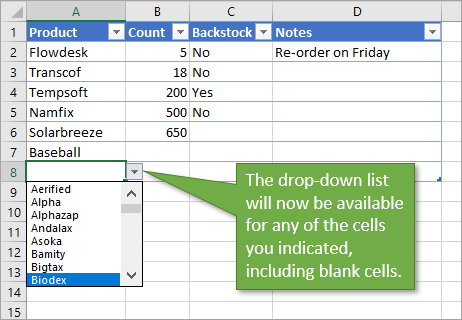
It's also worth noting that you can copy and paste Data Validation from one cell to another just as you would copy and paste normal values and formatting. 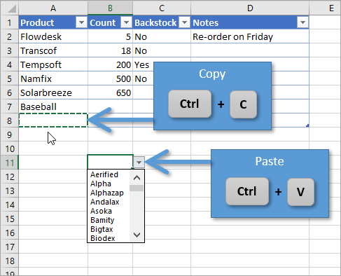 Handling Errors and Invalid Inputs
What happens when we enter a value into a cell that has a Data Validation List, but that value is not one of the options in the list? That depends on the Error Alert settings, which we have control of. 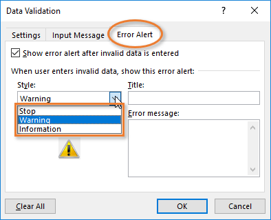
To change the kind of message the user receives when they enter an extraneous value, you can go back to the Data Validation window. Under the Error Alert tab, you can find three options: Stop, Warning, and Information. You’ll also notice that there are fields where you can change the title of the error message and the text of the message itself, so that when the user enters data that’s not part of your validation list, they will receive an alert that’s worded in the way you want it to appear. Here is an explanation of each Error Alert Style: Stop StyleWhen the user types an invalid entry, an error message will appear that gives the option to either retype the entry or cancel the attempt. The message looks like this:  Warning Style
The Warning style displays a message that gives the user a choice to allow an entry that isn’t on the preset list. 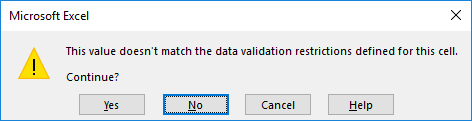 Information Style
The Information style displays a message that automatically allows the entry no matter what the value is. The user is presented with informative text about validation rules. 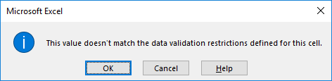 Error Checking Alert
When any invalid entry is made in a cell, the error checking alert will appear in the cell. The error is indicated with the green triangle in the top-left corner of the cell. Clicking the Error Box button will allow you to see more info about data validation error. You can select “Display Type Information” from the list to see the cause of the error. 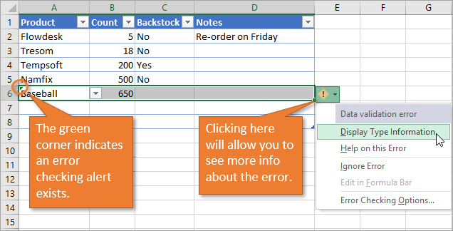
Disable Error Alerts Another option under the Error Alert tab is to uncheck the box that says, “Show error alert after invalid data is entered.” This allows any value to be entered into the cell, and no message box will appear. 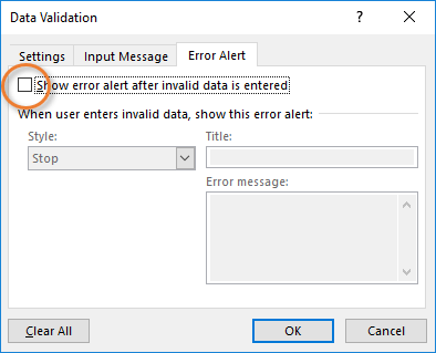 Adding New Data to the Source Range of the List
Adding new options to our drop-down list is possible, but it isn't automatic when we add new items the bottom of our source list. We need to tell Excel what our new extended source range is. You can do that in the Data Validation window by just typing in the new range, or re-selecting the range to include the new data. (See the section above entitled “Create a Drop-Down List from a Range of Values” for how to select your range.) The great thing is that we don't have to redefine these settings for each cell that has Data Validation. The “Apply these changes to all other cells with the same settings” checkbox does this for us. When you click the checkbox, the other cells will selected in the background. This gives you a visual indication of what will be updated. 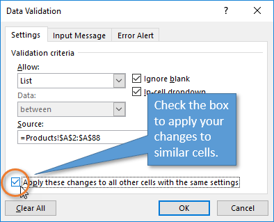
Then press OK. Any cells that shared the same data validation settings will now include the updated changes that you’ve made. There is a way to automate the process so that any change you make to the source data instantly updates your drop-down list. It involves using Excel tables and named ranges. You can find out how in this post: How to Add New Rows to Drop-down Lists Automatically – Dynamic Data Validation Lists Removing Data Validation from a CellGetting rid of a Data Validation list is simple. Open the Data Validation window and click the Clear All button. 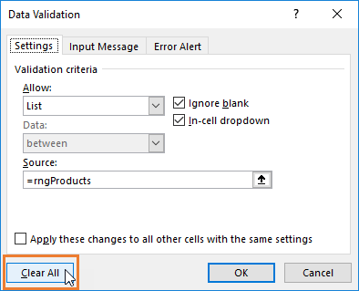
If you want to clear the validation settings from other cells with the same settings, make sure to click that checkbox before hitting the Clear All button. Make Your Workbooks InteractiveData Validation lists are a great tool to add to your Excel toolbelt. They help us keep our data clean and make our spreadsheets easier to use. We can use them as the source of lookup formulas to create interactive financial models and reports. I will do some follow-up posts with these techniques as well. Once you feel comfortable with drop-down lists, you may want to try dependent (also called cascading) lists. These are lists that change depending on what you've already chosen in another list. For example, you may create a list of car brands, like Toyota, Ford, and Honda. Then you can have a second list of car models that populates with specific options depending on what you choose in the first list. If you choose Toyota in the first list, you might see Corolla, Camry, and Tacoma in the second. But if you go back to the first list and choose Ford, the options in the second list can change to Mustang, Explorer, and Focus. Learn how to create dependent cascading lists here. If you have any questions or comments about how to use drop-down lists, don’t hesitate to leave a comment below. Thanks! 😊 |
【本文地址】