| 【机器学习算法笔记系列】逻辑回归(LR)算法详解和实战 | 您所在的位置:网站首页 › 惩罚逻辑回归有哪些 › 【机器学习算法笔记系列】逻辑回归(LR)算法详解和实战 |
【机器学习算法笔记系列】逻辑回归(LR)算法详解和实战
|
逻辑回归(LR)算法概述
逻辑回归(Logistic Regression)是用于处理因变量为分类变量的回归问题,常见的是二分类或二项分布问题,也可以处理多分类问题,它实际上是属于一种分类方法。 逻辑回归算法原理 预测函数和决策边界逻辑回归的预测函数可以表示为: 同理,对于非线性可分的情况,我们只需要引入多项式特征就可以很好的去做分类预测,如下图: 前面我们介绍线性回归模型时,给出了线性回归的代价函数的形式(误差平方和函数),具体形式如下: 为了可以更加方便的进行后面的参数估计求解,我们合并成一个公式: 和线性回归类似,我们使用梯度下降算法来求解逻辑回归模型的参数。代价函数梯度求解过程为: L1正则化和L2正则化可以看做是损失函数的惩罚项。所谓『惩罚』是指对损失函数中的某些参数做一些限制。对于线性回归模型,使用L1正则化的模型建叫做Lasso回归,使用L2正则化的模型叫做Ridge回归(岭回归)。 L1正则化和L2正则化的说明如下: L1正则化是指权值向量w中各个元素的绝对值之和,通常表示为: ∣ ∣ w ∣ ∣ 1 ||w||_1 ∣∣w∣∣1L2正则化是指权值向量w中各个元素的平方和然后再求平方根(可以看到Ridge回归的L2正则化项有平方符号),通常表示为: ∣ ∣ w ∣ ∣ 2 ||w||_2 ∣∣w∣∣2那添加L1和L2正则化有什么用? L1正则化可以产生稀疏权值矩阵(会让模型参数Θ稀疏化,即让模型参数向量里为0的元素尽量多),即产生一个稀疏模型,可以用于特征选择。L2正则化会让模型参数尽可能小,但不会为0(即尽量让每个特征对预测值都有一些小的贡献),可以防止模型过拟合(overfitting);一定程度上,L1也可以防止过拟合。因为下文逻辑回归实战中,利用l1作为正则项,这里我讲一下l1作为正则项的用途: 特征选择: 它会让模型参数向量里的元素为0的点尽量多,因此可以排除那些对特征值没有什么影响的特征,从而简化问题。所以l1范数解决过拟合的措施,实际上是减少特征数量。可解释性:模型参数向量稀疏化后,只会留下那些对特征值有重要影响的特征,这样我们就容易解释模型的因果关系,在下文的乳腺癌检测实战中,可以看到l1作为正则项的作用。由此可见,l1范数作为正则项,更多的是一个分析工具,适合用来对模型求解,它会把不重要的特征直接去除。大部分情况下,我们解决过拟合问题,还是选择l2范数作为正则项。 算法优缺点 优点 计算代价不高,训练速度较快,容易理解实现。LR在时间和内存需求上相当高效。它可以应用于分布式数据,并且还有在线算法实现,用较少的资源处理大型数据。模型的可解释性非常好,从特征的权重可以看到不同的特征对最后结果的影响。LR对于数据中小噪声的鲁棒性很好,并且不会受到轻微的多重共线性的特别影响。 缺点 准确率并不是很高。因为形式非常的简单(类似于线性模型),很难去拟合数据的真实分布。很难处理数据不平衡的问题。处理非线性数据较麻烦。逻辑回归在不引入其他方法的情况下,只能处理线性可分的数据,或者进一步说,处理二分类的问题 。对模型中自变量多重共线性较为敏感,需要利用因子分析或者变量聚类分析等手段来选择代表性的自变量,以减少候选变量之间的相关性。 Python实践scikit-learn中提供了一个LogisticRegression类来实现逻辑回归模型。LogisticRegression 其原型为:sklearn.linear_model.LogisticRegression(penalty=’l2’, dual=False, tol=0.0001, C=1.0, fit_intercept=True, intercept_scaling=1, class_weight=None, random_state=None, solver=’warn’, max_iter=100, multi_class=’warn’, verbose=0, warm_start=False, n_jobs=None) 参数penalty:str,指定正则化策略。 l2:l2正则化l1:l1正则化dual:bool:如果为True,则求解对偶形式(只在penalty="l2"且solver="liblinear"有对偶形式);如果为False,则求解原始形式。 C:float,指定罚项系数的倒数。如果它的值越小,则正则化项越大。 fit_intercept:bool,指定是否需要计算b值,如果为False,那么不会计算b值(模型会假设数据已经中心化了) intercept_scaling:float,只有当solver="liblinear"才有意义。当采用fit_intercept时,相当于人造一个特征出来,该特征恒为1,其权重为b。在计算正则化项的时候,该人造特征也被考虑了。为了降低这个人造特征的影响,需要提供intercept_scaling。 class_weight:dict或字符串'balanced' 如果为dict:字典给出每个分类的权重,如{class_label: weight}。如果为字符串balanced:则每个分类的权重与该分类在样本集中出现的概率成反比。如果未指定:每个分类的权重都为1。max_iter:int,指定最大迭代次数。 random_state:int,RandomState实例或None: 如果为int:指定随机数生成器的种子。如果为RandomState实例:指定随机数生成器。如果为None:使用默认的随机数生成器。solver:str,指定求解最优化问题的算法。 newton-cg:使用牛顿法。lbfgs:使用L-BFGS拟牛顿法。liblinear:使用liblinear。sag:使用Stochastic Average Gradient descent算法。 注意:对于小规模的数据集,liblinear比较适用;对于大规模的数据集,sag比较适用。newton-cg、lbfgs、sag只处理penalty=l2的情况。tol:float,指定判断迭代收敛与否的阈值。 multi_class:str,指定对于多分类问题的策略。 ovr:采用one-vs-rest策略。multinomial:直接采用多分类逻辑回归策略。verbose:int,用于开启/关闭迭代中间输出日志功能。 warm_start:bool,如果为True,那么使用前一次训练结果继续训练。否则从头开始训练。 n_jobs:int,指定任务并行时的CPU数量。如果为-1则使用所有可用CPU。 属性coef_:权重向量 intercept_:b值 n_iter_:实际迭代次数 方法fit(X, y[, sample_weight]):训练模型。 predict(X):用模型进行预测,返回预测值。 predict_log_proba(X):返回一个数组,数组的元素依次是X预测为各个类别的概率的对数值。 predict_proba(X):返回一个数组,数组的元素依次是X预测为各个类别的概率值。 score(X, y[, sample_weight]:返回在(X, y)上预测的准确率。 逻辑回归实战—乳腺癌检测本文使用逻辑回归算法解决乳腺癌检测问题。scikit-learn中自带一个乳腺癌数据集,为了方便起见,我们直接使用,读者也可直接在网上下载。乳腺癌数据集地址 首先,我们加载数据,输出数据形状和特征。以查看数据: __author__ = "fpZRobert" """ 逻辑回归实战—乳腺癌预测 """ from sklearn.datasets import load_breast_cancer """ 加载数据 """ cancer = load_breast_cancer() X = cancer.data y = cancer.target print("Shape of X: {0}; positive example: {1}; negative: {2}".format(X.shape, y[y==1].shape[0], y[y==0].shape[0])) # 查看数据的形状和类别分布 print("Cancer data feature name: ", cancer.feature_names) # 查看数据的特征 Out: Shape of X: (569, 30); positive example: 357; negative: 212 Cancer data feature name: ['mean radius' 'mean texture' 'mean perimeter' 'mean area' 'mean smoothness' 'mean compactness' 'mean concavity' 'mean concave points' 'mean symmetry' 'mean fractal dimension' 'radius error' 'texture error' 'perimeter error' 'area error' 'smoothness error' 'compactness error' 'concavity error' 'concave points error' 'symmetry error' 'fractal dimension error' 'worst radius' 'worst texture' 'worst perimeter' 'worst area' 'worst smoothness' 'worst compactness' 'worst concavity' 'worst concave points' 'worst symmetry' 'worst fractal dimension']我们可以看到,数据集总共有569个样本,每个样本有30个特征,其中357个阳性(y=1)样本,212个阴性(y=0)样本。从我们打印出来的特征可以看出,有些指标属于“复合”指标,即由其他的指标经过运算得到的。比如密实度,是由周长和面积计算出来的。这是实际工程应用中常用的特征提取手段:提取特征时,不妨从事务的内在逻辑关系入手,分析已有特征之间的关系,从而构造出新的特征。 回到我们讨论的乳腺癌数据集,实际上它只关注10个特征,然后又构造了每个特征的标准差及最大值,这样每个特征就又衍生出两个特征,所以总共就有了30个特征,这里我们介绍下这10个特征: 特征含义radius半径,即病灶中心点离边界的平均距离texture纹理,灰度值的标准偏差perimeter周长,即病灶的大小area面积,也是反映病灶大小的一个指标smoothness平滑度,即半径的变化幅度compactness密实度,周长的平方除以面积的商concavity凹度,凹陷部分轮廓的严重程度concave points凹点,凹陷轮廓的数量symmetry对称性fractal dimension分形维度把数据集划分为训练集和测试集(划分比例一般80%用于训练,20%用于测试): """ 构造训练集和测试集 """ from sklearn.model_selection import train_test_split X_train, X_test, y_train, y_test = train_test_split(X, y, test_size=0.2)使用逻辑回归算法对数据集进行拟合,并计算训练数据集的评分数据和测试数据集的评分数据: """ 模型训练 """ import numpy as np from sklearn.linear_model import LogisticRegression model = LogisticRegression() model.fit(X_train, y_train) train_score = model.score(X_train, y_train) test_score = model.score(X_test, y_test) print("train score: {train_score:.6f}; test score: {test_score:.6f}".format(train_score=train_score, test_score=test_score)) Out: train score: 0.956044; test score: 0.964912看起来和之前两篇博客的效果不一样,一上来效果就很不错,让我们看一下测试样本中,有哪些是预测正确的: """ 模型预测 """ y_pred = model.predict(X_test) print("matchs: {0}/{1}".format(np.equal(y_pred, y_test).shape[0], y_test.shape[0])) Out: matchs: 114/114一共114个样本,全部预测正确。这里抛出一个疑问:为什么全部预测正确,但test_score只有0.964912呢?其实,scikit-learn不是使用这个数据来计算分数的,因为这个数据不能完全反映误差情况,而是使用预测概率数据来计算模型得分的。 我们使用LogisticRegression模型的默认参数训练出来的模型,准确性看起来还不错,那么问题又来了,还有优化的空间吗? 首先,我们使用Pipeline来增加多项式特征,跟之前线性回归一样,这里不做过多介绍: """ 模型调优 """ from sklearn.preprocessing import PolynomialFeatures from sklearn.pipeline import Pipeline # 构建多项式模型 def polynomial_model(degree=1, **kwarg): polynomial_features = PolynomialFeatures(degree=degree, include_bias=False) logistic_regression = LogisticRegression(**kwarg) pipeline = Pipeline([("polynomial_feature", polynomial_features), ("logistic_regression", logistic_regression)]) return pipeline model = polynomial_model(degree=2, penalty="l1") model.fit(X_train, y_train) train_score_v2 = model.score(X_train, y_train) cv_score_v2 = model.score(X_test, y_test) print("train_score: {:.6f}, cv_score: {:.6f}".format(train_score_v2, cv_score_v2)) Out: train_score: 0.997802, cv_score: 0.982456可以看出,训练集评分和测试集评分都增加不少。为什么使用l1范数作为正则项呢?因为l1范数作为正则项,可以实现参数的稀疏化,即自动帮助我们选择那些对模型有关联的特征。我们可以观察一下有多少个特征没有被丢弃: logistic_regression = model.named_steps["logistic_regression"] print("model_parameters shape: {0}; count of non-zero element: {1}".format(logistic_regression.coef_.shape, np.count_nonzero(logistic_regression.coef_))) Out: model_parameters shape: (1, 495); count of non-zero element: 92逻辑回归模型的coef_属性中保存的就是模型参数,从输出结果看,增加到二阶多项式特征后,输入特征由原来的30个增加到495个,最终大多数特征被丢弃,只保留了94个有效特征。 学习曲线是模型最有效的诊断工具之一,首先我们画出L1范数作为正则项所对应的一阶和二阶多项式的学习曲线和L2范数作为正则项所对应的一阶和二阶多项式的学习曲线: """ 绘制学习曲线 """ import matplotlib.pyplot as plt from sklearn.model_selection import ShuffleSplit from sklearn.model_selection import learning_curve # 绘制学习曲线 def plot_learning_curve(plt, estimator, title, X, y, ylim=None, cv=None, n_jobs=1, train_sizes=np.linspace(.1, 1.0, 5)): plt.title(title) if ylim is not None: plt.ylim(*ylim) plt.xlabel("Training examples") plt.ylabel("Score") train_sizes, train_scores, test_scores = learning_curve( estimator, X, y, cv=cv, n_jobs=n_jobs, train_sizes=train_sizes) train_scores_mean = np.mean(train_scores, axis=1) train_scores_std = np.std(train_scores, axis=1) test_scores_mean = np.mean(test_scores, axis=1) test_scores_std = np.std(test_scores, axis=1) plt.grid() plt.fill_between(train_sizes, train_scores_mean - train_scores_std, train_scores_mean + train_scores_std, alpha=0.1, color="r") plt.fill_between(train_sizes, test_scores_mean - test_scores_std, test_scores_mean + test_scores_std, alpha=0.1, color="g") plt.plot(train_sizes, train_scores_mean, 'o--', color="r", label="Training score") plt.plot(train_sizes, test_scores_mean, 'o-', color="g", label="Cross-validation score") plt.legend(loc="best") return plt # 绘制L1范数作为正则化项所对应的一阶和二阶多项式的学习曲线 cv = ShuffleSplit(n_splits=10, test_size=0.2, random_state=0) title = "Learning Curves (degree={0}, penalty={1})" degrees = [1, 2] penalty = "l1" plt.figure(figsize=(12, 4), dpi=200) for i in range(len(degrees)): plt.subplot(1, len(degrees), i+1) plot_learning_curve(plt, polynomial_model(degree=degrees[i], penalty=penalty), title.format(degrees[i], penalty), X, y, (0.01, 1.01), cv) plt.show() # 绘制L2范数作为正则化项所对应的一阶和二阶多项式的学习曲线 penalty = "l2" plt.figure(figsize=(12, 4), dpi=200) plt.figure(figsize=(12, 4), dpi=200) for i in range(len(degrees)): plt.subplot(1, len(degrees), i+1) plot_learning_curve(plt, polynomial_model(degree=degrees[i], penalty=penalty, solver="lbfgs"), title.format(degrees[i], penalty), X, y, (0.01, 1.01), cv) plt.show()
全部代码: __author__ = "fpZRobert" """ 逻辑回归实战—乳腺癌预测 """ import numpy as np import matplotlib.pyplot as plt from sklearn.model_selection import ShuffleSplit from sklearn.model_selection import learning_curve from sklearn.linear_model import LogisticRegression from sklearn.preprocessing import PolynomialFeatures from sklearn.pipeline import Pipeline from sklearn.model_selection import train_test_split from sklearn.datasets import load_breast_cancer """ 加载数据 """ cancer = load_breast_cancer() X = cancer.data y = cancer.target print("Shape of X: {0}; positive example: {1}; negative: {2}".format(X.shape, y[y==1].shape[0], y[y==0].shape[0])) # 查看数据的形状和类别分布 print("Boston data feature name: ", cancer.feature_names) # 查看数据的特征 """ 构造训练集和测试集 """ X_train, X_test, y_train, y_test = train_test_split(X, y, test_size=0.2) """ 模型训练 """ model = LogisticRegression() model.fit(X_train, y_train) train_score = model.score(X_train, y_train) test_score = model.score(X_test, y_test) print("train score: {train_score:.6f}; test score: {test_score:.6f}".format(train_score=train_score, test_score=test_score)) """ 模型预测 """ y_pred = model.predict(X_test) print("matchs: {0}/{1}".format(np.equal(y_pred, y_test).shape[0], y_test.shape[0])) """ 模型调优 """ # 构建多项式模型 def polynomial_model(degree=1, **kwarg): polynomial_features = PolynomialFeatures(degree=degree, include_bias=False) logistic_regression = LogisticRegression(**kwarg) pipeline = Pipeline([("polynomial_feature", polynomial_features), ("logistic_regression", logistic_regression)]) return pipeline model = polynomial_model(degree=2, penalty="l1") model.fit(X_train, y_train) train_score_v2 = model.score(X_train, y_train) cv_score_v2 = model.score(X_test, y_test) print("train_score: {:.6f}, cv_score: {:.6f}".format(train_score_v2, cv_score_v2)) logistic_regression = model.named_steps["logistic_regression"] print("model_parameters shape: {0}; count of non-zero element: {1}".format(logistic_regression.coef_.shape, np.count_nonzero(logistic_regression.coef_))) """ 绘制学习曲线 """ # 绘制学习曲线 def plot_learning_curve(plt, estimator, title, X, y, ylim=None, cv=None, n_jobs=1, train_sizes=np.linspace(.1, 1.0, 5)): plt.title(title) if ylim is not None: plt.ylim(*ylim) plt.xlabel("Training examples") plt.ylabel("Score") train_sizes, train_scores, test_scores = learning_curve( estimator, X, y, cv=cv, n_jobs=n_jobs, train_sizes=train_sizes) train_scores_mean = np.mean(train_scores, axis=1) train_scores_std = np.std(train_scores, axis=1) test_scores_mean = np.mean(test_scores, axis=1) test_scores_std = np.std(test_scores, axis=1) plt.grid() plt.fill_between(train_sizes, train_scores_mean - train_scores_std, train_scores_mean + train_scores_std, alpha=0.1, color="r") plt.fill_between(train_sizes, test_scores_mean - test_scores_std, test_scores_mean + test_scores_std, alpha=0.1, color="g") plt.plot(train_sizes, train_scores_mean, 'o--', color="r", label="Training score") plt.plot(train_sizes, test_scores_mean, 'o-', color="g", label="Cross-validation score") plt.legend(loc="best") return plt # 绘制L1范数作为正则化项所对应的一阶和二阶多项式的学习曲线 cv = ShuffleSplit(n_splits=10, test_size=0.2, random_state=0) title = "Learning Curves (degree={0}, penalty={1})" degrees = [1, 2] penalty = "l1" plt.figure(figsize=(12, 4), dpi=200) for i in range(len(degrees)): plt.subplot(1, len(degrees), i+1) plot_learning_curve(plt, polynomial_model(degree=degrees[i], penalty=penalty), title.format(degrees[i], penalty), X, y, (0.01, 1.01), cv) plt.show() # 绘制L2范数作为正则化项所对应的一阶和二阶多项式的学习曲线 penalty = "l2" plt.figure(figsize=(12, 4), dpi=200) plt.figure(figsize=(12, 4), dpi=200) for i in range(len(degrees)): plt.subplot(1, len(degrees), i+1) plot_learning_curve(plt, polynomial_model(degree=degrees[i], penalty=penalty, solver="lbfgs"), title.format(degrees[i], penalty), X, y, (0.01, 1.01), cv) plt.show() 参考资料 细品 - 逻辑回归(LR)机器学习中正则化项L1和L2的直观理解 |
 举一个例子,假设我们有许多样本,并在图中表示出来了,并且假设我们已经通过某种方法求出了LR模型的参数(如下图):
  这时,直线上方所有样本都是正样本y=1,直线下方所有样本都是负样本y=0。因此我们可以把这条直线成为决策边界。
 值得注意的一点,决策边界并不是训练集的属性,而是假设本身和参数的属性。因为训练集不可以定义决策边界,它只负责拟合参数;而只有参数确定了,决策边界才得以确定。
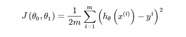 逻辑回归也可以视为一个广义的线性模型,那么线性模型中应用最广泛的代价函数-误差平方和函数,可不可以应用到逻辑回归呢?其实是不可以的,原因在于Sigmoid函数是一个复杂的非线性函数,我们将逻辑回归的假设函数带入上式中,得到J(Θ)是一个非凸函数,如下图:
  由上图可知,函数包含多个局部极小值点,使用梯度下降法求解损失函数最小值时,可能导致函数最后结果并非总是全局最小。所以,我们需要为逻辑回归找到一个凸代价函数,最常用的损失函数就是对数损失函数,对数损失函数可以为LR提供一个凸的代价函数,这样有利于使用梯度下降对参数求解。具体公式如下:
 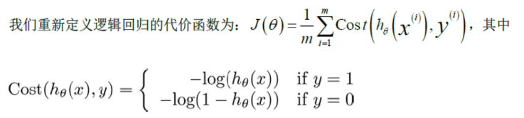 对于惩罚函数Cost的两种情况如下图所示:
  回顾成本的定义,成本是预测值与真实值的差异。当差异越大时,成本越大,模型受到的“惩罚”也越严重。如上左图所示,当y=1时,随着h(x)的值(预测为1的概率)越来越大,预测值越来越接近真实值,其成本也越来越小。如上右图所示,当y=0时,随着h(x)的值(预测为1的概率)越来越大,预测值越来越偏离真实值,其成本越来越大。
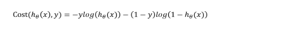 因此,我们的代价函数最终形式为:
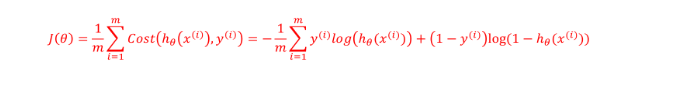
 最终推导出来的梯度下降算法公式为:
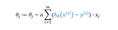
 正则化具体解释请参照:机器学习中正则化项L1和L2的直观理解
 从上图可以看出,使用多项式并使用L1范数作为正则化项的模型最优,因为它训练样本评分和交叉验证样本评分都很高。但从图中不难发现,训练样本和交叉样本之间的间隙还比较大,可以采集更多的有效数据进一步拟合模型,提高模型预测效果。
【本文地址】