零基础入门金融风控之贷款违约预测挑战赛

2023-04-01 16:55| 来源: 网络整理| 查看: 265

零基础入门金融风控之贷款违约预测挑战赛赛题理解

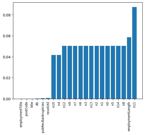
赛题以金融风控中的个人信贷为背景，要求选手根据贷款申请人的数据信息预测其是否有违约的可能，以此判断是否通过此项贷款，这是一个典型的分类问题。通过这道赛题来引导大家了解金融风控中的一些业务背景，解决实际问题，帮助竞赛新人进行自我练习、自我提高。

项目地址：https://github.com/datawhalechina/team-learning-data-mining/tree/master/FinancialRiskControl

比赛地址：https://tianchi.aliyun.com/competition/entrance/531830/introduction

数据形式

对于训练集数据来说，其中有特征如下：

id 为贷款清单分配的唯一信用证标识loanAmnt 贷款金额term 贷款期限（year）interestRate 贷款利率installment 分期付款金额grade 贷款等级subGrade 贷款等级之子级employmentTitle 就业职称employmentLength 就业年限（年）homeOwnership 借款人在登记时提供的房屋所有权状况annualIncome 年收入verificationStatus 验证状态issueDate 贷款发放的月份purpose 借款人在贷款申请时的贷款用途类别postCode 借款人在贷款申请中提供的邮政编码的前3位数字regionCode 地区编码dti 债务收入比delinquency_2years 借款人过去2年信用档案中逾期30天以上的违约事件数ficoRangeLow 借款人在贷款发放时的fico所属的下限范围ficoRangeHigh 借款人在贷款发放时的fico所属的上限范围openAcc 借款人信用档案中未结信用额度的数量pubRec 贬损公共记录的数量pubRecBankruptcies 公开记录清除的数量revolBal 信贷周转余额合计revolUtil 循环额度利用率，或借款人使用的相对于所有可用循环信贷的信贷金额totalAcc 借款人信用档案中当前的信用额度总数initialListStatus 贷款的初始列表状态applicationType 表明贷款是个人申请还是与两个共同借款人的联合申请earliesCreditLine 借款人最早报告的信用额度开立的月份title 借款人提供的贷款名称policyCode 公开可用的策略_代码=1新产品不公开可用的策略_代码=2n系列匿名特征匿名特征n0-n14，为一些贷款人行为计数特征的处理

还有一列为目标列isDefault代表是否违约。

预测指标

赛题要求采用AUC作为评价指标。

具体算法导入相关库 import pandas as pd import numpy as np from sklearn import metrics import matplotlib.pyplot as plt from sklearn.metrics import roc_auc_score, roc_curve, mean_squared_error,mean_absolute_error, f1_score import lightgbm as lgb import xgboost as xgb from sklearn.ensemble import RandomForestRegressor as rfr from sklearn.linear_model import LinearRegression as lr from sklearn.model_selection import KFold, StratifiedKFold,GroupKFold, RepeatedKFold import warnings warnings.filterwarnings('ignore') #消除warning 读入数据 train_data = pd.read_csv("train.csv") test_data = pd.read_csv("testA.csv") print(train_data.shape) print(test_data.shape)

(800000, 47) (200000, 47)

数据处理

由于等下需要对特征进行变化，因此我先将训练集和测试集堆叠在一起，一起处理才方便，再加入一列作为区分即可。

target = train_data["isDefault"] train_data["origin"] = "train" test_data["origin"] = "test" del train_data["isDefault"] data = pd.concat([train_data, test_data], axis = 0, ignore_index = True) data.shape

(1000000, 47)

那么接下来就是对data进行处理，可以先看看其大致的信息：

data.info() RangeIndex: 1000000 entries, 0 to 999999 Data columns (total 47 columns): # Column Non-Null Count Dtype --- ------ -------------- ----- 0 id 1000000 non-null int64 1 loanAmnt 1000000 non-null float64 2 term 1000000 non-null int64 3 interestRate 1000000 non-null float64 4 installment 1000000 non-null float64 5 grade 1000000 non-null object 6 subGrade 1000000 non-null object 7 employmentTitle 999999 non-null float64 8 employmentLength 941459 non-null object 9 homeOwnership 1000000 non-null int64 10 annualIncome 1000000 non-null float64 11 verificationStatus 1000000 non-null int64 12 issueDate 1000000 non-null object 13 purpose 1000000 non-null int64 14 postCode 999999 non-null float64 15 regionCode 1000000 non-null int64 16 dti 999700 non-null float64 17 delinquency_2years 1000000 non-null float64 18 ficoRangeLow 1000000 non-null float64 19 ficoRangeHigh 1000000 non-null float64 20 openAcc 1000000 non-null float64 21 pubRec 1000000 non-null float64 22 pubRecBankruptcies 999479 non-null float64 23 revolBal 1000000 non-null float64 24 revolUtil 999342 non-null float64 25 totalAcc 1000000 non-null float64 26 initialListStatus 1000000 non-null int64 27 applicationType 1000000 non-null int64 28 earliesCreditLine 1000000 non-null object 29 title 999999 non-null float64 30 policyCode 1000000 non-null float64 31 n0 949619 non-null float64 32 n1 949619 non-null float64 33 n2 949619 non-null float64 34 n3 949619 non-null float64 35 n4 958367 non-null float64 36 n5 949619 non-null float64 37 n6 949619 non-null float64 38 n7 949619 non-null float64 39 n8 949618 non-null float64 40 n9 949619 non-null float64 41 n10 958367 non-null float64 42 n11 912673 non-null float64 43 n12 949619 non-null float64 44 n13 949619 non-null float64 45 n14 949619 non-null float64 46 origin 1000000 non-null object dtypes: float64(33), int64(8), object(6) memory usage: 358.6+ MB

最重要的是对缺失值和异常值的处理，那么来看看哪些特征的缺失值和异常值最多：

missing = data.isnull().sum() / len(data) missing = missing[missing > 0 ] missing.sort_values(inplace = True) x = np.arange(len(missing)) fig, ax = plt.subplots() ax.bar(x,missing) ax.set_xticks(x) ax.set_xticklabels(list(missing.index), rotation = 90, fontsize = "small")

异常值

可以发现那些匿名特征的异常值都是很多的，还有employmentLength特征的异常值也很多。后续会进行处理。

另外，还有很多特征并不是能够直接用来训练的特征，因此需要对其进行处理，比如grade、subGrade、employmentLength、issueDate、earliesCreditLine，需要进行预处理.

print(sorted(data['grade'].unique())) print(sorted(data['subGrade'].unique())) ['A', 'B', 'C', 'D', 'E', 'F', 'G'] ['A1', 'A2', 'A3', 'A4', 'A5', 'B1', 'B2', 'B3', 'B4', 'B5', 'C1', 'C2', 'C3', 'C4', 'C5', 'D1', 'D2', 'D3', 'D4', 'D5', 'E1', 'E2', 'E3', 'E4', 'E5', 'F1', 'F2', 'F3', 'F4', 'F5', 'G1', 'G2', 'G3', 'G4', 'G5']

那么现在先对employmentLength特征进行处理：

data['employmentLength'].value_counts(dropna=False).sort_index() 1 year 65671 10+ years 328525 2 years 90565 3 years 80163 4 years 59818 5 years 62645 6 years 46582 7 years 44230 8 years 45168 9 years 37866 'booster': 'gbtree', 'objective': 'binary:logistic', 'eval_metric': 'auc', 'gamma': 1, 'min_child_weight': 1.5, 'max_depth': 5, 'lambda': 10, 'subsample': 0.7, 'colsample_bytree': 0.7, 'colsample_bylevel': 0.7, 'eta': 0.04, 'tree_method': 'exact', 'seed': 1, 'nthread': 36, "verbosity": 1, } folds = StratifiedKFold(n_splits=5, shuffle=True, random_state=1) valid_xgb = np.zeros(len(x_train)) predict_xgb = np.zeros(len(x_test)) for fold_, (train_idx,valid_idx) in enumerate(folds.split(x_train, y_train)): print("当前第{}折".format(fold_ + 1)) train_data_now = xgb.DMatrix(x_train.iloc[train_idx], y_train[train_idx]) valid_data_now = xgb.DMatrix(x_train.iloc[valid_idx], y_train[valid_idx]) watchlist = [(train_data_now,"train"), (valid_data_now, "valid_data")] xgb_model = xgb.train(dtrain = train_data_now, num_boost_round = 3000, evals = watchlist, early_stopping_rounds = 500, verbose_eval = 500, params = xgb_params) valid_xgb[valid_idx] =xgb_model.predict(xgb.DMatrix(x_train.iloc[valid_idx]), ntree_limit = xgb_model.best_ntree_limit) predict_xgb += xgb_model.predict(xgb.DMatrix(x_test),ntree_limit = xgb_model.best_ntree_limit) / folds.n_splits

放一下部分训练过程吧：

当前第5折 [0] train-auc:0.69345 valid_data-auc:0.69341 [500] train-auc:0.73811 valid_data-auc:0.72788 [1000] train-auc:0.74875 valid_data-auc:0.73066 [1500] train-auc:0.75721 valid_data-auc:0.73194 [2000] train-auc:0.76473 valid_data-auc:0.73266 [2500] train-auc:0.77152 valid_data-auc:0.73302 [2999] train-auc:0.77775 valid_data-auc:0.73307

那么接下来的模型融合我就采用了简单的逻辑回归：

# 模型融合 train_stack = np.vstack([valid_lgb, valid_xgb]).transpose() test_stack = np.vstack([predict_lgb, predict_xgb]).transpose() folds_stack = RepeatedKFold(n_splits = 5, n_repeats = 2, random_state = 1) valid_stack = np.zeros(train_stack.shape[0]) predict_lr2 = np.zeros(test_stack.shape[0]) for fold_, (train_idx, valid_idx) in enumerate(folds_stack.split(train_stack, target)): print("当前是第{}折".format(fold_+1)) train_x_now, train_y_now = train_stack[train_idx], target.iloc[train_idx].values valid_x_now, valid_y_now = train_stack[valid_idx], target.iloc[valid_idx].values lr2 = lr() lr2.fit(train_x_now, train_y_now) valid_stack[valid_idx] = lr2.predict(valid_x_now) predict_lr2 += lr2.predict(test_stack) / 10 print("score:{:

【本文地址】

公司简介

联系我们