实用篇

2024-06-09 17:40| 来源: 网络整理| 查看: 265

本文主要是为了快速的了解t-sne和如何快速使用！

简要了解TSNE

TSNE，降维方法之一。降维在机器学习中非常重要。这是因为如果使用高维数据创建模型，则很容易欠拟合。换句话说，有太多无用的数据需要学习。可以通过从各种数据中仅选择最重要的数据在模型中使用它，也可以使用多个数据创建新数据并使其低维。无论如何，有必要将此类高维数据转换为低维数据。这称为降维。（还有其他方法可以创建要素，例如“特征消除”和“特征选择”。降维方法有两种类型：线性方法（主成分分析（PCA），独立成分分析，线性判别分析等）和非线性方法（歧管，自动编码器等）。TSNE是多种方法之一。它从SNE（随机邻居嵌入）演变为t-SNE（t分布随机邻居嵌入），然后发展到UMAP（均匀流形近似和投影）

TSNE是由T和SNE组成，T分布和随机近邻嵌入(Stochastic neighbor Embedding).TSNE是一种可视化工具，将高位数据降到2-3维，然后画成图。t-SNE是目前效果最好的数据降维和可视化方法t-SNE的缺点是：占用内存大，运行时间长。

t-sne实现过程：How to Use t-SNE Effectively (distill.pub)

T-SNE算法步骤找出高维空间中相邻点之间的成对相似性。根据高维空间中点的成对相似性，将高维空间中的每个点映射到低维映射。使用基于Kullback-Leibler散度(KL散度)的梯度下降找到最小化条件概率分布之间的不匹配的低维数据表示。使用Student-t分布计算低维空间中两点之间的相似度。

案例1：随机生成数据并进行降维类型1 import matplotlib.pyplot as plt from sklearn.manifold import TSNE tsne = TSNE(n_components=2) x = [[1,2,2],[2,2,2],[3,3,3]] y = [1,0,2]#y是x对应的标签 x_tsne = tsne.fit_transform(x) plt.scatter(x_tsne[:,0],x_tsne[:,1],c=y) plt.show()

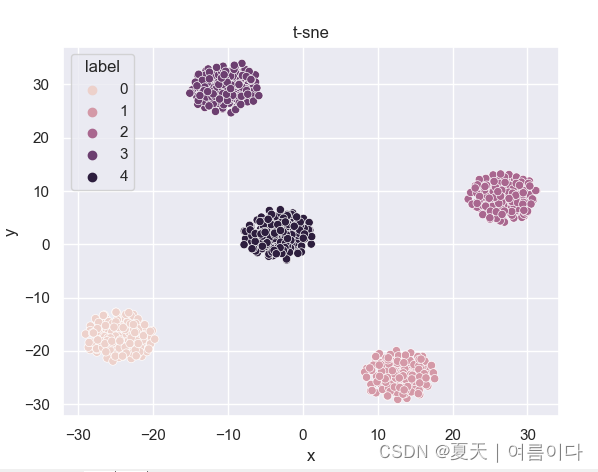
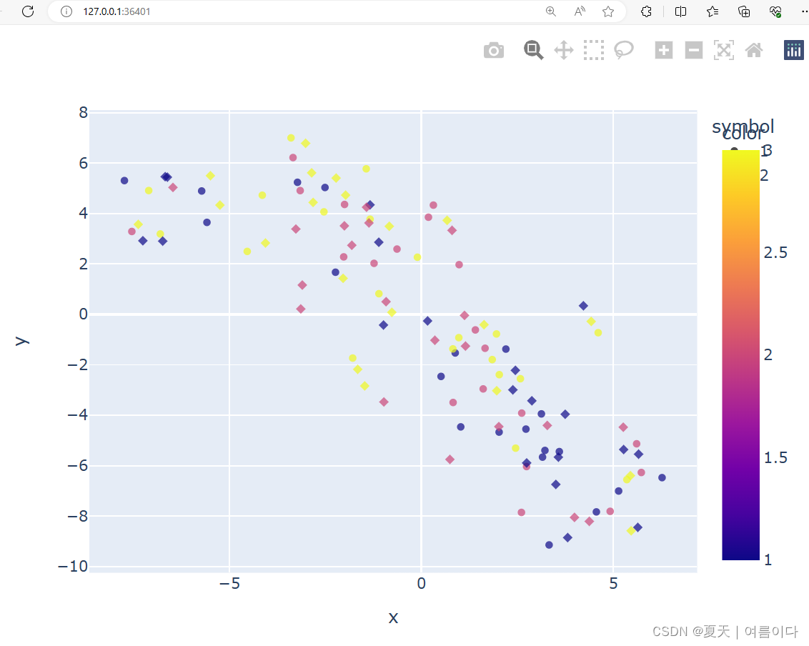
类型2 #pip install pandas import pandas as pd import matplotlib.pyplot as plt import seaborn as sns sns.set() def get_data(): """生成聚类数据""" from sklearn.datasets import make_blobs x_value, y_value = make_blobs(n_samples=1000, n_features=40, centers=3, ) return x_value, y_value def plot_xy(x_values, label, title): """绘图""" df = pd.DataFrame(x_values, columns=['x', 'y']) df['label'] = label sns.scatterplot(x="x", y="y", hue="label", data=df) plt.title(title) plt.show() def main(): x_value, y_value = get_data() # PCA 降维 from sklearn.decomposition import PCA pca = PCA(n_components=2) x_pca = pca.fit_transform(x_value) plot_xy(x_pca, y_value, "PCA") # t-sne 降维 from sklearn.manifold import TSNE tsne = TSNE(n_components=2) x_tsne = tsne.fit_transform(x_value) plot_xy(x_tsne, y_value, "t-sne") if __name__ == '__main__': main()

案例2：用t-SNE降维查看分类效果

读取数据集的特征及标签，并进行降维画图

2.1.计算机视觉类 2.1.1.MNIST数据集上实现t-SNE的Python代码 #! pip install sklearn #! pip install seaborn #! pip install matplotlib from sklearn.datasets import load_digits from sklearn.manifold import TSNE import seaborn as sns from matplotlib import pyplot as plt # 0-9的数字数据 data = load_digits() embeddings = TSNE().fit_transform(digits.data)#t-SNE降维，默认降为二维 vis_x = embeddings[:, 0]#0维 vis_y = embeddings[:, 1]#1维 index0 = [i for i in range(len(digits.target)) if digits.target == 0] index1 = [i for i in range(len(digits.target)) if digits.target == 1] index2 = [i for i in range(len(digits.target)) if digits.target == 2] index3 = [i for i in range(len(digits.target)) if digits.target == 3] index4 = [i for i in range(len(digits.target)) if digits.target == 4] index5 = [i for i in range(len(digits.target)) if digits.target == 5] index6 = [i for i in range(len(digits.target)) if digits.target == 6] index7 = [i for i in range(len(digits.target)) if digits.target == 7] index8 = [i for i in range(len(digits.target)) if digits.target == 8] index9 = [i for i in range(len(digits.target)) if digits.target == 9] colors=['b', 'c', 'y', 'm', 'r', 'g', 'k','yellow','yellowgreen','wheat'] plt.scatter(vis_x[index0], vis_y[index0], c=colors[0], cmap='brg', marker='h',label='0') plt.scatter(vis_x[index1], vis_y[index1], c=colors[1], cmap='brg',marker='',label='5') plt.scatter(vis_x[index6], vis_y[index6], c=colors[6], cmap='brg',marker='^',label='6') plt.scatter(vis_x[index7], vis_y[index7], c=colors[7], cmap='brg',marker='d',label='7') plt.scatter(vis_x[index8], vis_y[index8], c=colors[8], cmap='brg',marker='s',label='8') plt.scatter(vis_x[index9], vis_y[index9], c=colors[9], cmap='brg',marker='o',label='9') plt.title(u't-SNE') plt.legend() plt.show() 2.1.2.动物(Animals10)数据集上的可视化

使用 Animals10 数据集。它包含 10 种不同动物的图片：猫、狗、鸡、牛、马、羊、松鼠、大象、蝴蝶和蜘蛛。

数据集下载地址：Animals-10 (kaggle.com)

代码还在优化中。。。

import #设置随机种子 seed = 10 random.seed(seed) torch.manual_seed(seed) np.random.seed(seed) # ResNet101 网络提取图片特征 # Define the architecture by modifying resnet. # Original code is here http://tiny.cc/8zpmmz class ResNet101(models.ResNet): def __init__(self, num_classes=1000, pretrained=True, **kwargs): # Start with the standard resnet101 super().__init__( block=models.resnet.Bottleneck, layers=[3, 4, 23, 3], num_classes=num_classes, **kwargs ) if pretrained: state_dict = load_state_dict_from_url( models.resnet.model_urls['resnet101'], progress=True ) self.load_state_dict(state_dict) # Reimplementing forward pass. # Replacing the forward inference defined here # http://tiny.cc/23pmmz def _forward_impl(self, x): # Standard forward for resnet x = self.conv1(x) x = self.bn1(x) x = self.relu(x) x = self.maxpool(x) x = self.layer1(x) x = self.layer2(x) x = self.layer3(x) x = self.layer4(x) # Notice there is no forward pass through the original classifier. x = self.avgpool(x) x = torch.flatten(x, 1) return x #存储推按2048特征 # initialize our implementation of ResNet model = ResNet101(pretrained=True) model.eval() for batch in tqdm(dataloader, desc='Running the model inference'): images = batch['image'].to(device) labels += batch['label'] image_paths += batch['image_path'] output = model.forward(images) current_outputs = output.cpu().numpy() features = np.concatenate((outputs, current_outputs)) tsne = TSNE(n_components=2).fit_transform(features) # scale and move the coordinates so they fit [0; 1] range def scale_to_01_range(x): # compute the distribution range value_range = (np.max(x) - np.min(x)) # move the distribution so that it starts from zero # by extracting the minimal value from all its values starts_from_zero = x - np.min(x) # make the distribution fit [0; 1] by dividing by its range return starts_from_zero / value_range # extract x and y coordinates representing the positions of the images on T-SNE plot tx = tsne[:, 0] ty = tsne[:, 1] tx = scale_to_01_range(tx) ty = scale_to_01_range(ty) # 绘制2D点，每个点的颜色与类标签对应 # initialize a matplotlib plot fig = plt.figure() ax = fig.add_subplot(111) # for every class, we'll add a scatter plot separately for label in colors_per_class: # find the samples of the current class in the data indices = [i for i, l in enumerate(labels) if l == label] # extract the coordinates of the points of this class only current_tx = np.take(tx, indices) current_ty = np.take(ty, indices) # convert the class color to matplotlib format color = np.array(colors_per_class[label], dtype=np.float) / 255 # add a scatter plot with the corresponding color and label ax.scatter(current_tx, current_ty, c=color, label=label) # build a legend using the labels we set previously ax.legend(loc='best') # finally, show the plot plt.show() 2.2.语音类 2.2.1在语音数据集上利用tsne进行可视化

要求数据类别和数据是相同的，需要修改部分数据

from matplotlib import pyplot as plt import matplotlib.cm as cm import fnmatch import os import numpy as np import librosa import matplotlib.pyplot as plt import librosa.display from sklearn.manifold import TSNE import json # Importing library import csv import numpy as np import pandas as pd import matplotlib.pyplot as plt import seaborn as sns import glob path = "/workspace/emo-vits/dataset/p225" files = [] for root, dirnames, filenames in os.walk(path): for filename in fnmatch.filter(filenames, '*.wav'): files.append(os.path.join(root, filename)) print("found %d .wav files"%(len(files))) def get_features(y, sr): y = y[0:sr] # analyze just first second S = librosa.feature.melspectrogram(y, sr=sr, n_mels=128) log_S = librosa.amplitude_to_db(S, ref=np.max) mfcc = librosa.feature.mfcc(S=log_S, n_mfcc=13) delta_mfcc = librosa.feature.delta(mfcc, mode='nearest') delta2_mfcc = librosa.feature.delta(mfcc, order=2, mode='nearest') feature_vector = np.concatenate((np.mean(mfcc,1), np.mean(delta_mfcc,1), np.mean(delta2_mfcc,1))) feature_vector = (feature_vector-np.mean(feature_vector)) / np.std(feature_vector) return feature_vector feature_vectors = [] sound_paths = [] for i,f in enumerate(files): if i % 100 == 0: print("get %d of %d = %s"%(i+1, len(files), f)) y, sr = librosa.load(f) feat = get_features(y, sr) feature_vectors.append(feat) sound_paths.append(f) print("calculated %d feature vectors"%len(feature_vectors)) model = TSNE(n_components=2, learning_rate=150, perplexity=30, verbose=2, angle=0.1).fit_transform(feature_vectors) symbol=[] symbol=[1]*1400 x=[2]*1400 symbol.extend(x) # classes file=[1,2,3] color=[] for i in file: x=[i]*20 color.extend(x) color.extend(color) print(len(color)) x_axis=model[:,0] y_axis=model[:,1] import plotly.express as px fig = px.scatter(x=x_axis, y=y_axis,color=color,symbol=symbol,opacity=0.7) fig.show() ''' # load 2D vector x = np.load(path) #使用np.ravel将向量展平为一维数组。 #x = np.ravel(x) print(x.shape) # 2D vector -> high-dis tsne= TSNE(n_components=2).fit_transform(x) X_embedded = tsne.fit_transform(X) # high-dis -> 2D vector line_vector = 0 for i in range(0, 222): line_vector = x[i] print(line_vector)'''

参考文献

【1】Clustering with KMeans, PCA, TSNE | Kaggle

【2】[차원축소/시각화 방법] TSNE - Python 에서 T-SNE를 이용하는 방법 :: The Yellow Lion King 데이터와 함께 살아가기 (tistory.com) 【3】t-SNE 개념과 사용법 - gaussian37

【4】 Audio Dataset Analysis-4 | Kaggle

【本文地址】

公司简介

联系我们