【数据分析】重庆二手房市场分析

2022-10-17 05:09| 来源: 网络整理| 查看: 265

笔者未系统性学习数据分析，本系列文章仅为笔者选修课《数据科学导论》大作业内容。如有纰漏，敬请指出数据预处理

使用one-hot编码修改特征position,decoration，仅考虑position，去掉district字段。

district = pd.get_dummies(result['position'], prefix='地段') data = pd.concat([result, district], axis=1) dec = pd.get_dummies(result['decoration'], prefix='装修') data = pd.concat([data, dec], axis=1) data.drop(['district','position','community','decoration','LATB','LNGB'], axis=1, inplace=True) price = data['unit_price'] data.drop(labels=['unit_price'], axis=1,inplace = True) data.insert(0, 'unit_price', price) print(data.head())

输出：

unit_price area year 东东北东南北南西西北 ... 地段_鸿恩寺地段_黄桷坪 \ 0 8538 134.70 2006 0 0 0 0 0 0 1 ... 0 0 1 10953 105.00 2006 1 0 0 0 0 0 0 ... 0 0 2 11026 95.23 2006 0 0 0 0 0 0 0 ... 0 0 3 11342 82.00 2006 0 0 0 0 0 0 0 ... 0 0 4 11476 81.04 2008 0 0 0 0 1 0 0 ... 0 0 地段_黄泥磅地段_龙头寺地段_龙洲湾地段_龙溪装修_其他装修_毛坯装修_简装装修_精装 0 0 0 0 0 0 1 0 0 1 0 0 0 0 0 0 0 1 2 0 0 0 0 0 0 1 0 3 0 0 0 0 0 0 0 1 4 0 0 0 0 0 0 0 1 [5 rows x 106 columns]

分割数据与标准化处理：

#确定数据中的特征与标签 x = data.as_matrix()[:,1:] y = data.as_matrix()[:,0].reshape(-1,1) #数据分割，随机采样25%作为测试样本，其余作为训练样本 from sklearn.model_selection import train_test_split x_train, x_test, y_train, y_test = train_test_split(x, y, random_state=40, test_size=0.25) #数据标准化处理 from sklearn.preprocessing import StandardScaler ss_x = StandardScaler() ss_y = StandardScaler() x_train = ss_x.fit_transform(x_train) x_test = ss_x.transform(x_test) y_train = ss_y.fit_transform(y_train) y_test = ss_y.transform(y_test)模型预测from sklearn.linear_model import LinearRegression from sklearn.ensemble import RandomForestRegressor from sklearn.svm import SVR from sklearn.metrics import r2_score #使用线性回归模型预测 lr = LinearRegression() lr.fit(x_train, y_train) lr_y_predict = lr.predict(x_test) #使用SVM模型预测 svr = SVR() svr.fit(x_train, y_train) svr_y_predict = svr.predict(x_test) #使用随机森林模型预测 rf = RandomForestRegressor() rf.fit(x_train, y_train) rf_y_predict = rf.predict(x_test) print("线性回归 R方：", r2_score(y_test, lr_y_predict)) print("SVM R方：", r2_score(y_test, svr_y_predict)) print("随机森林 R方：", r2_score(y_test, rf_y_predict))

输出：

线性回归 R方： 0.4384207215126369 SVM R方： 0.5075938836179383 随机森林 R方： 0.714459871333186

绘图：

plt.rcParams['figure.figsize'] = (10,3) # 设置figure_size尺寸 plt.subplots_adjust(wspace=0.25) plt.subplot(131) plt.scatter(ss_y.inverse_transform(y_test),ss_y.inverse_transform(lr_y_predict),s=2) plt.xlim(0,35000) plt.ylim(0,35000) plt.xlabel('真实值') plt.ylabel('预测值') x = np.linspace(0,35000,1000) plt.plot(x,x,color='red',linestyle='--',linewidth=2) plt.title('线性回归模型') plt.subplot(132) plt.scatter(ss_y.inverse_transform(y_test),ss_y.inverse_transform(svr_y_predict),s=2) plt.xlim(0,35000) plt.ylim(0,35000) plt.xlabel('真实值') plt.ylabel('预测值') x = np.linspace(0,35000,1000) plt.plot(x,x,color='red',linestyle='--',linewidth=2) plt.title('SVM模型') plt.subplot(133) plt.scatter(ss_y.inverse_transform(y_test), ss_y.inverse_transform(rf_y_predict),s=2) plt.xlim(0,35000) plt.ylim(0,35000) plt.xlabel('真实值') plt.ylabel('预测值') x = np.linspace(0,35000,1000) plt.plot(x,x,color='red',linestyle='--',linewidth=2) plt.title('随机森林模型') plt.show()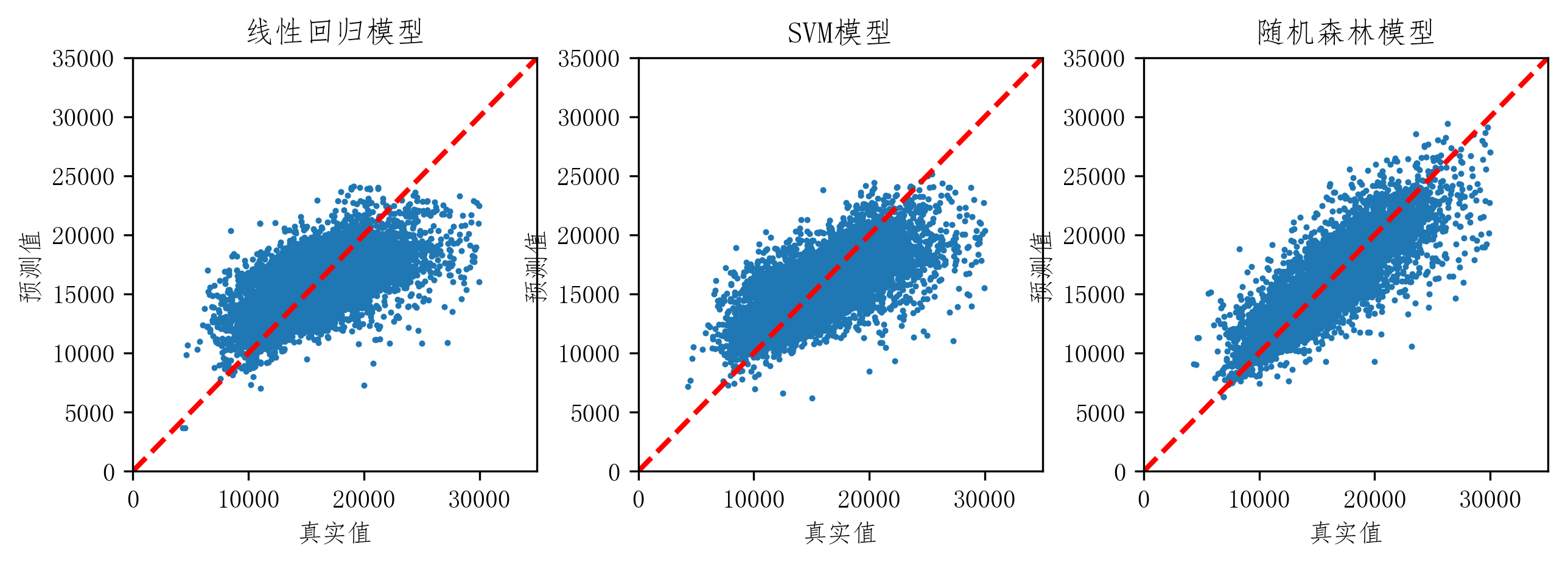

房源描述分析

链家上对房源还有一个title字段，是房主对房源的描述。这些描述对房价应该也有一点影响，但是并不好进行处理，下面仅做所有房源的描述的词云。

from os import path from scipy.misc import imread import matplotlib.pyplot as plt import jieba from wordcloud import WordCloud, ImageColorGenerator text_path = 'titles.txt' # 设置要分析的文本路径 text = open(text_path,'rb').read() def jiebaclearText(text): mywordlist = [] seg_list = jieba.cut(text, cut_all=False) liststr = "/ ".join(seg_list) for myword in liststr.split('/'): if len(myword.strip()) > 1: mywordlist.append(myword) return ''.join(mywordlist) text = jiebaclearText(text) back_coloring_path = "logo2.png" font_path = 'C:/Windows/Fonts/Deng.ttf' back_coloring = imread(back_coloring_path) # 设置词云属性 wc = WordCloud( font_path=font_path, # 设置字体 background_color="white", # 背景颜色 mask=back_coloring, # 设置背景图片 random_state=42, margin=2 ) wc.generate(text) plt.figure() plt.imshow(wc) plt.axis("off") plt.show() wc.to_file('output.png')

【本文地址】

公司简介

联系我们