TensorFlow

2023-09-17 19:28| 来源: 网络整理| 查看: 265

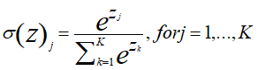
对数几率回归解决的是二分类的问题，对于多个选项的问题，我们可以使用softmax函数，它是对数几率回归在 N 个可能不同的值上的推广。神经网络的原始输出不是一个概率值，实质上只是输入的数值做了复杂的加权和（乘以w+b）与非线性处理之后的一个值而已，那么如何将这个输出变为概率分布？ -这就是Softmax层的作用了

softmax要求每个样本必须属于某个类别，且所有可能的样本均被覆盖 1.softmax个样本分量之和为 1 （1）概率之和为1.预测一个人来自广州，还是广西，上海等地，，这是个多分类问题，softmax分类之后，谁的概率大，预测值就是谁，当只有两个值的时候，->2。 2.当只有两个类别时，与对数几率回归完全相同

tf.keras交叉熵

在tf.keras里，对于多分类问题我们使用

categorical_crossentropy 和

sparse_categorical_crossentropy #顺序数字编码时使用

来计算softmax交叉熵

Fashion MNIST 数据集

Fashion MNIST 的作用是成为经典 MNIST 数据集的简易替换， MNIST 数据集包含手写数字（0、1、2 等）的图像，这些图像的格式与本节课中使用的服饰图像的格式相同。

Fashion MNIST 比常规 MNIST手写数据集更具挑战性。这两个数据集都相对较小，用于验证某个算法能否如期正常运行。它们都是测试和调试代码的良好起点。

Fashion MNIST 数据集包含 70000 张灰度图像，涵盖 10 个类别。

我们将使用 60000 张图像训练网络，并使用 10000 张图像评估经过学习的网络分类图像的准确率。

可以从 TensorFlow 直接访问 Fashion MNIST，只需导入和加载数据即可

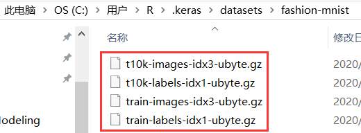
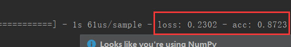
Fashion MNIST会自动去下载那些图片与数据，这里直接导入，就不用慢慢下载了

multi-classification.py 代码如下：

import tensorflow as tf #print('Tensorflow Version:{}'.format(tf.__version__)) import pandas as pd import numpy as np import matplotlib.pyplot as plt (train_image,train_lable),(test_image,test_label)=tf.keras.datasets.fashion_mnist.load_data() #将fashion_mnist直接加进来 train_image.shape train_lable.shape train_image.shape,train_lable.shape plt.imshow(train_image[0]) #plt.show() #print(train_image[0]) #print(np.max(train_image[0])) #print(train_lable) #数据归一化 train_image=train_image/255 test_image =test_image/255 #print(train_image.shape) #(60000, 28, 28) model=tf.keras.Sequential() #Dense是将一个一维的数据映射另一个一维数据上（张量为一维） #而这个是二维的，需要flatten转化为一维的 # model.add(tf.keras.layers.Flatten(input_shape=(28,28))) #扁平成28*28的向量 # model.add(tf.keras.layers.Dense(128,activation='relu')) # #输出 # model.add(tf.keras.layers.Dense(10,activation='softmax')) #变成长度为10个概率值,softmax把它激活成概率分布 # #编译模型 # model.compile(optimizer='adam', # loss='sparse_categorical_crossentropy', #顺序数字编码时使用 # metrics=['acc']) #度量正确率 # #训练 # model.fit(train_image,train_lable,epochs=5) #评价 #model.evaluate(test_image,test_label) #print(train_lable) #独热编码 # beijing [1,0,0] # shanghai [0,1,0] # shenzhen [0,0,1] train_lable_onehot=tf.keras.utils.to_categorical(train_lable) # print(train_lable_onehot) # # print(train_lable_onehot[-1]) model.add(tf.keras.layers.Flatten(input_shape=(28,28))) #扁平成28*28的向量 model.add(tf.keras.layers.Dense(128,activation='relu')) #输出 model.add(tf.keras.layers.Dense(10,activation='softmax')) #变成长度为10个概率值,softmax把它激活成概率分布 #编译模型 model.compile(optimizer='adam', loss='categorical_crossentropy', #顺序数字编码时使用 metrics=['acc']) #度量正确率 #训练 model.fit(train_image,train_lable_onehot,epochs=5) predict = model.predict(test_image) print(test_image.shape) predict.shape print(predict[0]) print(np.argmax(predict[0])) #预测最大值 #看看是不是最大值 print(test_label[0])

其中的一张图片

第10000张

独热编码

print(train_lable)

打印出： [9 0 0 ... 3 0 5]

print(train_lable_onehot)

print(train_lable_onehot[-1])

打印出： [0. 0. 0. 0. 0. 1. 0. 0. 0. 0.]

【本文地址】

公司简介

联系我们