| Mathematica数学学习快速入门指南 | 您所在的位置:网站首页 › wolfram怎么算定积分 › Mathematica数学学习快速入门指南 |
Mathematica数学学习快速入门指南
|
阿里网盘pdf文件分享 目录1 进入数学快速入门官网文档2 面向数学学习的快速入门指南2.1 内容输入2.2 分数与小数2.3 变量与函数2.4 代数2.5 二维绘图2.6 几何2.7 三角函数2.8 极坐标2.9 指数和对数2.10 极限2.11 导数2.12 积分2.13 序列、求和与级数2.14 更多二维绘图2.15 三维绘图2.16 多变量微积分2.17 矢量分析与可视化2.18 微分方程2.19 复分析2.20 矩阵与线性代数2.21 离散数学2.22 概率2.23 统计2.24 绘制数据与最佳拟合曲线2.25 群论2.26 数学难题2.27 交互模型2.28 数学排版显示2.29 笔记本文档2.30 云部署 1 进入数学快速入门官网文档
进入到
拉到网页最下面
点击面向数学学习的快速入门指南即可进入官方数学学习教程 2 面向数学学习的快速入门指南 2.1 内容输入在网络或桌面 Wolfram 笔记本中,只须输入内容,然后按下 SHIFT+ENTER 进行计算: In[1]:= Out[1]=

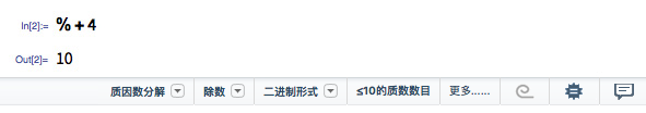
In[n] 和 Out[n] 标示出相邻的输入和输出. % 符号指代最近的输出: In[1]:= Out[1]=
 In[2]:=
 Out[2]=

执行完计算以后,建议栏会提供下一步计算的建议:
在数学运算中可以使用标准符号: (用空格或 * 表示乘法,不要用字符 “x”.) In[1]:= Out[1]=

用小括号(不是中括号或大括号)显示不同层次的组合: In[2]:= Out[2]=

Wolfram 语言有大约 6,000 个内置函数,涵盖了各个方面的数学知识. 用逗号分隔内置函数的参数,并将其置于方括号内: In[1]:= GCD[12, 15]
Out[1]= GCD[12, 15]
Out[1]=

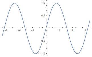
如果不知道使用哪个函数,在行的开始处键入 = 即可进行自然语言输入: In[2]:=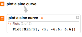 plot a sine curve
Out[2]= plot a sine curve
Out[2]=
Lists 表示一些项的集合,用 { ... } 表示: In[1]:= {1, 2, 3} {x, y, z} {1, 2, 3} {x, y, z}
列表是有序的. 可以包含数字、变量、计算,甚至是其他列表: 许多运算是被应用到每个元素上的: In[2]:= {1, 2, 3} + 2
Out[2]= {1, 2, 3} + 2
Out[2]=

从 1 开始,可以用 [[ ... ]] 来提取列表的元素: In[3]:= {a, b, c, d}[[3]]
Out[3]= {a, b, c, d}[[3]]
Out[3]=

通过使用如 Range 这样的函数可以轻松构建列表: In[1]:= Range[10]
Out[1]= Range[10]
Out[1]=
 2.2 分数与小数
在 Wolfram 语言中,精确输入(如分数)会提供精确的输出: (用 CTRL+ / 输入分数.) In[1]:= 1/4 + 1/3
Out[1]= 1/4 + 1/3
Out[1]=

用 Together 写成最小公分母的形式: In[2]:= Together[1/a + 1/b]
Out[2]= Together[1/a + 1/b]
Out[2]=

任何含有小数的输入给出近似输出: In[1]:= .25 + 1/3
Out[1]= .25 + 1/3
Out[1]=

用 N 得到结果的数字近似值: In[2]:= N[1/4 + 1/7]
Out[2]= N[1/4 + 1/7]
Out[2]=

指定所示答案的准确度: In[3]:= N[1/4 + 1/7, 10]
Out[3]= N[1/4 + 1/7, 10]
Out[3]=

有些数字表示成 ScientificForm 形式会更合适: In[1]:= ScientificForm[0.00123]
Out[1]= ScientificForm[0.00123]
Out[1]=

在适合的情况下,系统自动使用 ScientificForm 形式: In[2]:= N[100!]
Out[2]= N[100!]
Out[2]=
 2.3 变量与函数
变量以字母开头,可以含有数字: (最好是用小写字母,把大写开头留给内置函数.) In[1]:= a1/2
Out[1]= a1/2
Out[1]=

两个变量或数字间的空格表示相乘: (换句话说,“a b” 表示 a 乘以 b,而 “ab” 则为变量 ab.) In[2]:= a b + 5 x x
Out[2]= a b + 5 x x
Out[2]=

用 /. 和 -> 在表达式中进行替代操作: (可用 -> 输入 “rule” -> .) In[3]:= 1 + 2 x /. x -> 2
Out[3]= 1 + 2 x /. x -> 2
Out[3]=

用 = 符号赋值: In[1]:= x = 2
Out[1]= x = 2
Out[1]=

在表达式和命令中使用变量: In[2]:= 1 + 2 x
Out[2]= 1 + 2 x
Out[2]=

清除赋值,x 保持未计算状态: In[3]:= Clear[x] 1 + 2 x
Out[3]= Clear[x] 1 + 2 x
Out[3]=

用 f[x_]:= 来定义自己的函数: In[1]:= f[x_] := 1 + 2 x f[x_] := 1 + 2 x
x_ 表示 x 是一个模式,任何值都可以取代它. := 表示在计算时传递给 f 的任何参数将被代入右侧: In[2]:= f[2]
Out[2]= f[2]
Out[2]=
 2.4 代数
可以因式分解或展开代数表达式: (用 CTRL+6 输入排版式指数.) In[1]:= Factor[x^2 + 2 x + 1]
Out[1]= Factor[x^2 + 2 x + 1]
Out[1]=

Wolfram 语言用 == (两个等号)检测是否相等: In[1]:= 2 + 2 == 4
Out[1]= 2 + 2 == 4
Out[1]=

用 == 把代数表达式组合在一起表示方程: In[2]:= 1 + z == 15
Out[2]= 1 + z == 15
Out[2]=

像 Solve 这样的命令给出的是方程的精确解: In[1]:= Solve[x^2 + 5 x - 6 == 0, x]
Out[1]= Solve[x^2 + 5 x - 6 == 0, x]
Out[1]=
如果想要得到近似结果,用 NSolve: In[2]:= NSolve[7 x^2 + 3 x - 5 == 0, x]
Out[2]= NSolve[7 x^2 + 3 x - 5 == 0, x]
Out[2]=
以列表形式把一个方程组传递给函数: In[3]:= Solve[{x^2 + 5 == y, 7 x - 5 == y}, {x, y}]
Out[3]= Solve[{x^2 + 5 == y, 7 x - 5 == y}, {x, y}]
Out[3]=
求方程的根: (|| 是 Or 的符号.) In[1]:= Roots[x^2 + 3 x - 4 == 0, x]
Out[1]= Roots[x^2 + 3 x - 4 == 0, x]
Out[1]=

如果一个多项式不易被因式分解,近似结果可能更有用: In[2]:= NRoots[360 + 234 x - 1051 x^2 + 11 x^3 + 304 x^4 - 20 x^5 == 0, x]
Out[2]= NRoots[360 + 234 x - 1051 x^2 + 11 x^3 + 304 x^4 - 20 x^5 == 0, x]
Out[2]=

Reduce 命令可把一组不等式化简成简单的形式: (可键入 "Expressions"]
Out[1]=
或对绘图进行填充来查看曲线下的面积: In[2]:= Plot[1/x, {x, -3, 3}, Filling -> Axis]
Out[2]= Plot[1/x, {x, -3, 3}, Filling -> Axis]
Out[2]=
用 Show 来组合不同的绘图类型: In[1]:= Show[{Plot[x^2 + 2, {x, -3, 3}], RegionPlot[2 x > y - 3, {x, -3, 3}, {y, 0, 9}]}]
Out[1]= Show[{Plot[x^2 + 2, {x, -3, 3}], RegionPlot[2 x > y - 3, {x, -3, 3}, {y, 0, 9}]}]
Out[1]=
 2.6 几何
Graphics 命令可以生成各种各样的二维形状: In[1]:= Graphics[Disk[]]
Out[1]= Graphics[Disk[]]
Out[1]=

许多几何对象接受一系列坐标(列表)作为参数: In[2]:= Graphics[Rectangle[{0, 0}, {4, 2}]]
Out[2]= Graphics[Rectangle[{0, 0}, {4, 2}]]
Out[2]=

与指令一起以列表形式传递参数,把图形组合在一起并改变它们的样式: In[3]:= Graphics[{Green, Rectangle[{0, 0}, {2, 2}], Red, Disk[]}]
Out[3]= Graphics[{Green, Rectangle[{0, 0}, {2, 2}], Red, Disk[]}]
Out[3]=
用诸如 SASTriangle 这样的命令生成三角形: (键入 ESC+deg+ESC 可输入 ° 符号.) In[1]:= tr = SASTriangle[1, 90 \[Degree], 2]
Out[1]= tr = SASTriangle[1, 90 \[Degree], 2]
Out[1]=
可以直接算出如面积这样的属性: In[2]:= Area[tr]
Out[2]= Area[tr]
Out[2]=

把该表达式传递给 Graphics: In[3]:= Graphics[tr]
Out[3]= Graphics[tr]
Out[3]=

同样,可以用 Graphics3D 显示三维物体: In[1]:= Graphics3D[Ball[]]
Out[1]= Graphics3D[Ball[]]
Out[1]=
计算体积及其他属性: (如果没有给出参数,圆柱的半径为1,高度为 2.) In[2]:= Volume[Cylinder[]]
Out[2]= Volume[Cylinder[]]
Out[2]=

还可以用自然语言输入查找公式和其他信息: In[3]:= volume of a cone
Out[3]= volume of a cone
Out[3]=
系统还内置有几何变换,如 Rotate、Translate 和 Scale: In[1]:= Graphics[Rotate[Rectangle[], 45 \[Degree]]]
Out[1]= Graphics[Rotate[Rectangle[], 45 \[Degree]]]
Out[1]=
 2.7 三角函数
对于基本的三角函数,可以使用标准的缩写形式(首字母大写): In[1]:= Sin[x]/Cos[x] == Tan[x]
Out[1]= Sin[x]/Cos[x] == Tan[x]
Out[1]=

加上 “Arc” 求反函数: In[2]:= ArcTan[1]
Out[2]= ArcTan[1]
Out[2]=

在弧度表达式中使用 Pi: (键入 ESC+pi+ESC 来输入 π 字符.) In[1]:= Sin[\[Pi]/2]
Out[1]= Sin[\[Pi]/2]
Out[1]=

或输入 ESCd+eg+ESC 得到内置的 Degree 符号: In[2]:= Sin[90 \[Degree]]
Out[2]= Sin[90 \[Degree]]
Out[2]=

用恒等式自动展开(或化简)三角表达式: In[1]:= TrigExpand[Sin[2 x]]
Out[1]= TrigExpand[Sin[2 x]]
Out[1]=

因式分解三角多项式: In[2]:= TrigFactor[Cos[x]^2 - Sin[x]^2]
Out[2]= TrigFactor[Cos[x]^2 - Sin[x]^2]
Out[2]=
也可以使用像 Solve 这样的函数: In[1]:= Solve[Cos[x]^2 + Sin[x]^2 == x]
Out[1]= Solve[Cos[x]^2 + Sin[x]^2 == x]
Out[1]=

指定解的值域: In[2]:= Solve[{Tan[x] == 1, 0 < x < 2 Pi}]
Out[2]= Solve[{Tan[x] == 1, 0 < x < 2 Pi}]
Out[2]=
 2.8 极坐标
创建二维极坐标图: (键入 ESC+th+ESC 可得到 θ 符号.) In[1]:= PolarPlot[Sin[2 \[Theta]] + Cos[2 \[Theta]], {\[Theta], 0, 2 Pi}]
Out[1]= PolarPlot[Sin[2 \[Theta]] + Cos[2 \[Theta]], {\[Theta], 0, 2 Pi}]
Out[1]=
显示极坐标轴: In[2]:= PolarPlot[Sin[2 \[Theta]] + Cos[2 \[Theta]], {\[Theta], 0, 2 Pi}, PolarAxes -> Automatic, PolarTicks -> {0 \[Degree], 90 \[Degree], 180 \[Degree], 270 \[Degree]}]
Out[2]= PolarPlot[Sin[2 \[Theta]] + Cos[2 \[Theta]], {\[Theta], 0, 2 Pi}, PolarAxes -> Automatic, PolarTicks -> {0 \[Degree], 90 \[Degree], 180 \[Degree], 270 \[Degree]}]
Out[2]=
把直角坐标转换成极坐标: In[1]:= ToPolarCoordinates[{1, 1}]
Out[1]= ToPolarCoordinates[{1, 1}]
Out[1]=
 2.9 指数和对数
Wolfram 语言用 E 表示指数常数. Log 给出一个表达式的自然对数: In[1]:= Log[E^2]
Out[1]= Log[E^2]
Out[1]=

计算以 2 为基数的对数: In[2]:= Log[2, 64]
Out[2]= Log[2, 64]
Out[2]=

在对数刻度上绘图: In[1]:= LogPlot[E^x, {x, 1, 5}]
Out[1]= LogPlot[E^x, {x, 1, 5}]
Out[1]=
把两个坐标轴都设成对数刻度: In[2]:= LogLogPlot[x^2 + x^3, {x, 1, 100}]
Out[2]= LogLogPlot[x^2 + x^3, {x, 1, 100}]
Out[2]=
 2.10 极限
计算表达式的极限值: (键入 -> 可得到 符号.) In[1]:= Limit[(x^3 - 1)/(x - 1), x -> 1]
Out[1]= Limit[(x^3 - 1)/(x - 1), x -> 1]
Out[1]=

求 Infinity 处的极限: (键入 ESC+inf+ESC 可得到 ∞ 符号.) In[2]:= Limit[(2 x^3 - 1)/(5 x^3 + x - 1), x -> \[Infinity]]
Out[2]= Limit[(2 x^3 - 1)/(5 x^3 + x - 1), x -> \[Infinity]]
Out[2]=

还可以指定极限的方向. 设置为 1 时从左侧逼近极限: In[1]:= Limit[1/x, x -> 0, Direction -> 1]
Out[1]= Limit[1/x, x -> 0, Direction -> 1]
Out[1]=

设置为 -1 时从右侧逼近极限: In[2]:= Limit[1/x, x -> 0, Direction -> -1]
Out[2]= Limit[1/x, x -> 0, Direction -> -1]
Out[2]=

用 HoldForm 将表达式保持为未计算状态: (TraditionalForm 用传统的数学排版形式显示.) In[1]:= TraditionalForm[HoldForm[Limit[1/x, x -> Infinity]]]
Out[1]= TraditionalForm[HoldForm[Limit[1/x, x -> Infinity]]]
Out[1]=
 2.11 导数
用命令 D 计算导数: In[1]:= D[x^6, x]
Out[1]= D[x^6, x]
Out[1]=

或者使用角分符号: In[2]:= Sin'[x]
Out[2]= Sin'[x]
Out[2]=

对用户定义的函数求导: In[1]:= f[x_] := x^2 + 2 x + 1; f'[x]
Out[1]= f[x_] := x^2 + 2 x + 1; f'[x]
Out[1]=

绘制导数: In[2]:= Plot[{f[x], f'[x]}, {x, -3, 3}]
Out[2]= Plot[{f[x], f'[x]}, {x, -3, 3}]
Out[2]=
还可以多次求导: In[1]:= D[x^6, {x, 3}]
Out[1]= D[x^6, {x, 3}]
Out[1]=

或者多次使用 ' 符号: In[2]:= Sin''[x]
Out[2]= Sin''[x]
Out[2]=

和前面讨论过的主题一样,也可以通过自然语言输入得到微积分公式: In[1]:= product rule formula
Out[1]= product rule formula
Out[1]=
 2.12 积分
用 Integrate 计算积分: In[1]:= Integrate[8 x^4, x]
Out[1]= Integrate[8 x^4, x]
Out[1]=

或输入 ESC+intt+ESC 得到一个可填充的数学表达式: (如果想了解更多关于可填充表达式的信息,请参阅数学排版显示.) In[2]:= \[Integral]8 x^4 \[DifferentialD]x
Out[2]= \[Integral]8 x^4 \[DifferentialD]x
Out[2]=

对于定积分,输入 ESC+dintt+ESC 并指定上下限: In[1]:= \!\( \*SubsuperscriptBox[\(\[Integral]\), \(0\), \(\[Pi]\)]\(Sin[ x] \[DifferentialD]x\)\)
Out[1]= \!\( \*SubsuperscriptBox[\(\[Integral]\), \(0\), \(\[Pi]\)]\(Sin[ x] \[DifferentialD]x\)\)
Out[1]=

用 NIntegrate 来得到数值近似: In[2]:= NIntegrate[x^3 Sin[x] + 2 Log[3 x]^2, {x, 0, Pi}]
Out[2]= NIntegrate[x^3 Sin[x] + 2 Log[3 x]^2, {x, 0, Pi}]
Out[2]=
 2.13 序列、求和与级数
在 Wolfram 语言中,用列表表示整数序列. 用 Table 来定义一个简单的序列: In[1]:= Table[x^2, {x, 1, 7}]
Out[1]= Table[x^2, {x, 1, 7}]
Out[1]=
系统内置有大家熟知的序列: In[2]:= Table[Fibonacci[x], {x, 1, 7}]
Out[2]= Table[Fibonacci[x], {x, 1, 7}]
Out[2]=
用 RecurrenceTable 定义递归序列: (注意 {x,min,max} 表示法的使用.) In[1]:= RecurrenceTable[{a[x] == 2 a[x - 1], a[1] == 1}, a, {x, 1, 8}]
Out[1]= RecurrenceTable[{a[x] == 2 a[x - 1], a[1] == 1}, a, {x, 1, 8}]
Out[1]=
计算序列的 Total: In[2]:= Total[%]
Out[2]= Total[%]
Out[2]=

根据母函数计算序列的 Sum: In[1]:= Sum[i (i + 1), {i, 1, 10}]
Out[1]= Sum[i (i + 1), {i, 1, 10}]
Out[1]=

用 ESC+sumt+ESC 得到可填充的排版形式: In[2]:= \!\( \*UnderoverscriptBox[\(\[Sum]\), \(i = 1\), \(10\)]\(i \((i + 1)\)\)\)
Out[2]= \!\( \*UnderoverscriptBox[\(\[Sum]\), \(i = 1\), \(10\)]\(i \((i + 1)\)\)\)
Out[2]=

可以进行不定求和与多重求和计算: In[3]:= \!\( \*UnderoverscriptBox[\(\[Sum]\), \(i = 1\), \(n\)]\( \*UnderoverscriptBox[\(\[Sum]\), \(j = 1\), \(n\)]i\ j\)\)
Out[3]= \!\( \*UnderoverscriptBox[\(\[Sum]\), \(i = 1\), \(n\)]\( \*UnderoverscriptBox[\(\[Sum]\), \(j = 1\), \(n\)]i\ j\)\)
Out[3]=

计算序列的母函数: In[1]:= FindSequenceFunction[{2, 4, 6, 8}, n]
Out[1]= FindSequenceFunction[{2, 4, 6, 8}, n]
Out[1]=

生成几乎任意内置函数的组合的幂级数近似: In[1]:= Series[Exp[x^2], {x, 0, 8}]
Out[1]= Series[Exp[x^2], {x, 0, 8}]
Out[1]=
O[x]9 表示省略掉的更高次数的项;用 Normal 来截断这些项: In[2]:= Normal[%]
Out[2]= Normal[%]
Out[2]=
给定一个未知或未定义的函数,Series 返回用导数表示的幂级数: In[3]:= Series[2 f[x] - 3, {x, 0, 3}]
Out[3]= Series[2 f[x] - 3, {x, 0, 3}]
Out[3]=
系统可自动化简收敛级数: In[1]:= \!\( \*UnderoverscriptBox[\(\[Sum]\), \(n = 0\), \(\[Infinity]\)] \*SuperscriptBox[\(0.5\), \(n\)]\)
Out[1]= \!\( \*UnderoverscriptBox[\(\[Sum]\), \(n = 0\), \(\[Infinity]\)] \*SuperscriptBox[\(0.5\), \(n\)]\)
Out[1]=
 2.14 更多二维绘图
用 ParametricPlot 来绘制一组参数方程: In[1]:= ParametricPlot[{2 Cos[t] - Cos[2 t], 2 Sin[t] - Sin[2 t]}, {t, 0, 2 Pi}]
Out[1]= ParametricPlot[{2 Cos[t] - Cos[2 t], 2 Sin[t] - Sin[2 t]}, {t, 0, 2 Pi}]
Out[1]=
用多个变量绘制函数的 ContourPlot: In[1]:= ContourPlot[Sqrt[x^2 + y^2], {x, -1, 1}, {y, -1, 1}]
Out[1]= ContourPlot[Sqrt[x^2 + y^2], {x, -1, 1}, {y, -1, 1}]
Out[1]=
用 DensityPlot 绘制连续形式的图: In[2]:= DensityPlot[Sqrt[x^2 + y^2], {x, -1, 1}, {y, -1, 1}]
Out[2]= DensityPlot[Sqrt[x^2 + y^2], {x, -1, 1}, {y, -1, 1}]
Out[2]=
 2.15 三维绘图
Plot3D 可绘制三维的笛卡尔曲线或曲面: In[1]:= Plot3D[x^2 - y^2 , {x, -3, 3}, {y, -3, 3}]
Out[1]= Plot3D[x^2 - y^2 , {x, -3, 3}, {y, -3, 3}]
Out[1]=
用 ParametricPlot3D 绘制三维空间曲线: In[2]:= ParametricPlot3D[{Sin[u], Cos[u], u/10}, {u, 0, 20}]
Out[2]= ParametricPlot3D[{Sin[u], Cos[u], u/10}, {u, 0, 20}]
Out[2]=
如果想在球面坐标系中绘图,用 SphericalPlot3D: In[3]:= SphericalPlot3D[Sin[\[Theta]], {\[Theta], 0, Pi}, {\[Phi], 0, 2 Pi}]
Out[3]= SphericalPlot3D[Sin[\[Theta]], {\[Theta], 0, Pi}, {\[Phi], 0, 2 Pi}]
Out[3]=
RevolutionPlot3D 通过绕轴旋转一个表达式构建曲面: In[1]:= RevolutionPlot3D[x^4 - x^2, {x, -1, 1}]
Out[1]= RevolutionPlot3D[x^4 - x^2, {x, -1, 1}]
Out[1]=
 2.16 多变量微积分
D 可用于求偏导数,只需指定对哪个或哪些变量求导: In[1]:= D[x^3 z + 2 y^2 x + y z^3, y, z]
Out[1]= D[x^3 z + 2 y^2 x + y z^3, y, z]
Out[1]=

或使用 ∂ 符号: (键入 ESC+pd+ESC 可以输入 ∂,CTRL+- 产生下标.) In[2]:= \!\( \*SubscriptBox[\(\[PartialD]\), \(x, y\)]\(( \*SuperscriptBox[\(x\), \(2\)] - 2 x\ y + x\ y\ z)\)\)
Out[2]= \!\( \*SubscriptBox[\(\[PartialD]\), \(x, y\)]\(( \*SuperscriptBox[\(x\), \(2\)] - 2 x\ y + x\ y\ z)\)\)
Out[2]=

多重积分与单个积分的符号是一样的: (键入 ESC+int+ESC 可得到 ∫,用 ESC+dd+ESC 得到  \[Integral]\[Integral]\[Integral](x^2 + y^2 + z^2) \[DifferentialD]y \[DifferentialD]x \[DifferentialD]z
Out[1]= \[Integral]\[Integral]\[Integral](x^2 + y^2 + z^2) \[DifferentialD]y \[DifferentialD]x \[DifferentialD]z
Out[1]=
符号式结果常常相当复杂: In[2]:= \!\( \*SubsuperscriptBox[\(\[Integral]\), \(-1\), \(1\)]\( \*SubsuperscriptBox[\(\[Integral]\), \(-2\), \(x\)]\((x\ Sin[ \*SuperscriptBox[\(y\), \(2\)]] + y\ Cos[ \*SuperscriptBox[\(x\), \(2\)]])\) \[DifferentialD]y \ \[DifferentialD]x\)\)
Out[2]= \!\( \*SubsuperscriptBox[\(\[Integral]\), \(-1\), \(1\)]\( \*SubsuperscriptBox[\(\[Integral]\), \(-2\), \(x\)]\((x\ Sin[ \*SuperscriptBox[\(y\), \(2\)]] + y\ Cos[ \*SuperscriptBox[\(x\), \(2\)]])\) \[DifferentialD]y \ \[DifferentialD]x\)\)
Out[2]=
这种情况下,总可以通过使用 N 命令得到近似结果: In[3]:= N[%, 5]
Out[3]= N[%, 5]
Out[3]=
 2.17 矢量分析与可视化
在 Wolfram 语言中,用长度为 n 的列表表示 n 维矢量. 计算两个矢量的点积: In[1]:= {1, 2, 3}.{a, b, c}
Out[1]= {1, 2, 3}.{a, b, c}
Out[1]=

输入 ESC+cross+ESC 得到叉乘符号: In[2]:= {1, 2, c}\[Cross]{a, b, c}
Out[2]= {1, 2, c}\[Cross]{a, b, c}
Out[2]=
计算矢量的模: In[1]:= Norm[{1, 1, 1}]
Out[1]= Norm[{1, 1, 1}]
Out[1]=

求矢量在 x 轴上的投影: In[2]:= Projection[{8, 6, 7}, {1, 0, 0}]
Out[2]= Projection[{8, 6, 7}, {1, 0, 0}]
Out[2]=

求两个矢量的夹角: In[3]:= VectorAngle[{1, 0}, {0, 1}]
Out[3]= VectorAngle[{1, 0}, {0, 1}]
Out[3]=

计算矢量的梯度: (用 ESC+grad+ESC 输入 ∇ 符号.) In[1]:= \!\( \*SubscriptBox[\(\[Del]\), \({x, y}\)]\({ \*SuperscriptBox[\(x\), \(2\)] + y, x + \*SuperscriptBox[\(y\), \(2\)]}\)\)
Out[1]= \!\( \*SubscriptBox[\(\[Del]\), \({x, y}\)]\({ \*SuperscriptBox[\(x\), \(2\)] + y, x + \*SuperscriptBox[\(y\), \(2\)]}\)\)
Out[1]=

计算向量场的散度或旋度: In[2]:= Div[{f[x, y, z], g[x, y, z], h[x, y, z]}, {x, y, z}]
Out[2]= Div[{f[x, y, z], g[x, y, z], h[x, y, z]}, {x, y, z}]
Out[2]=

Wolfram 语言拥有适合于可视化向量场的二维和三维函数: In[1]:= VectorPlot[{y, -x}, {x, -3, 3}, {y, -3, 3}]
Out[1]= VectorPlot[{y, -x}, {x, -3, 3}, {y, -3, 3}]
Out[1]=
 In[2]:=
 VectorPlot3D[{y, -x, z}, {x, -3, 3}, {y, -3, 3}, {z, -3, 3}]
Out[2]= VectorPlot3D[{y, -x, z}, {x, -3, 3}, {y, -3, 3}, {z, -3, 3}]
Out[2]=
在切片曲面上绘制向量场: In[3]:= SliceVectorPlot3D[{y, -x, z}, "CenterPlanes", {x, -2, 2}, {y, -2, 2}, {z, -2, 2}]
Out[3]= SliceVectorPlot3D[{y, -x, z}, "CenterPlanes", {x, -2, 2}, {y, -2, 2}, {z, -2, 2}]
Out[3]=
 2.18 微分方程
Wolfram 语言可以求解常微分方程、偏微分方程和时滞微分方程 (ODE、PDE 和 DDE). DSolveValue 接受微分方程并返回通解: (C[1] 表示积分常数.) In[1]:= sol = DSolveValue[y'[x] + y[x] == x, y[x], x]
Out[1]= sol = DSolveValue[y'[x] + y[x] == x, y[x], x]
Out[1]=

用 /. 替换常数: In[2]:= sol /. C[1] -> 1
Out[2]= sol /. C[1] -> 1
Out[2]=

或为特解加上条件: In[3]:= DSolveValue[{y'[x] + y[x] == x, y[0] == -1}, y[x], x]
Out[3]= DSolveValue[{y'[x] + y[x] == x, y[0] == -1}, y[x], x]
Out[3]=

NDSolveValue 可求出数值解: In[1]:= NDSolveValue[{y'[x] == Cos[x^2], y[0] == 0}, y[x], {x, -5, 5}]
Out[1]= NDSolveValue[{y'[x] == Cos[x^2], y[0] == 0}, y[x], {x, -5, 5}]
Out[1]=
可直接绘制 InterpolatingFunction: In[2]:= Plot[%, {x, -5, 5}]
Out[2]= Plot[%, {x, -5, 5}]
Out[2]=
如果想要求解微分方程组,把所有方程和条件都放在列表中: (注意:换行符没有任何影响.) In[1]:= {xsol, ysol} = NDSolveValue[ {x'[t] == -y[t] - x[t]^2, y'[t] == 2 x[t] - y[t]^3, x[0] == y[0] == 1}, {x, y}, {t, 20}]
Out[1]= {xsol, ysol} = NDSolveValue[ {x'[t] == -y[t] - x[t]^2, y'[t] == 2 x[t] - y[t]^3, x[0] == y[0] == 1}, {x, y}, {t, 20}]
Out[1]=
用参数图可视化解: In[2]:= ParametricPlot[{xsol[t], ysol[t]}, {t, 0, 20}]
Out[2]= ParametricPlot[{xsol[t], ysol[t]}, {t, 0, 20}]
Out[2]=
 2.19 复分析
虚部单位  I^2
Out[1]= I^2
Out[1]=

许多运算可以自动处理复数: In[2]:= (1 + I) (2 - 3 I)
Out[2]= (1 + I) (2 - 3 I)
Out[2]=

展开复数表达式: In[1]:= ComplexExpand[Sin[x + I y]]
Out[1]= ComplexExpand[Sin[x + I y]]
Out[1]=
在指数形式和三角函数形式之间转换表达式: In[2]:= ExpToTrig[E^(I x)]
Out[2]= ExpToTrig[E^(I x)]
Out[2]=
 In[3]:=
 TrigToExp[%]
Out[3]= TrigToExp[%]
Out[3]=

输入 ESC+co+ESC 可得到 Conjugate 符号: In[1]:= (3 + 2 I)\[Conjugate]
Out[1]= (3 + 2 I)\[Conjugate]
Out[1]=

提取表达式的实部和虚部: In[2]:= ReIm[3 + 2 I]
Out[2]= ReIm[3 + 2 I]
Out[2]=

或求绝对值和辐角: In[3]:= AbsArg[(1 + I)]
Out[3]= AbsArg[(1 + I)]
Out[3]=

用 ParametricPlot 绘制保角映射: In[1]:= ParametricPlot[ReIm[E^(I \[Omega])], {\[Omega], 0, 2 \[Pi]}]
Out[1]= ParametricPlot[ReIm[E^(I \[Omega])], {\[Omega], 0, 2 \[Pi]}]
Out[1]=
在 PolarPlot 中使用 AbsArg: In[2]:= PolarPlot[AbsArg[E^(I \[Omega])], {\[Omega], 0, \[Pi]}]
Out[2]= PolarPlot[AbsArg[E^(I \[Omega])], {\[Omega], 0, \[Pi]}]
Out[2]=
用 DensityPlot 可视化复分量: In[3]:= DensityPlot[Im[ArcSin[(x + I y)^2]], {x, -2, 2}, {y, -2, 2}]
Out[3]= DensityPlot[Im[ArcSin[(x + I y)^2]], {x, -2, 2}, {y, -2, 2}]
Out[3]=
 2.20 矩阵与线性代数
Wolfram 语言用列表的列表表示矩阵: In[1]:= {{1, 2}, {3, 4}} {{1, 2}, {3, 4}}
输入一个表格,用 CTRL+ ENTER 输入行,用 CTRL+ , 输入列: In[2]:= { {a, b}, {c, d} }
Out[2]= { {a, b}, {c, d} }
Out[2]=

MatrixForm 将输出显示为一个矩阵: In[3]:= MatrixForm[{{a, b}, {c, d}}]
Out[3]= MatrixForm[{{a, b}, {c, d}}]
Out[3]=

可以用迭代函数构建矩阵: In[1]:= Table[x + y, {x, 1, 3}, {y, 0, 2}]
Out[1]= Table[x + y, {x, 1, 3}, {y, 0, 2}]
Out[1]=
或导入表示矩阵的数据: In[2]:= Import["data.csv"]
Out[2]= Import["data.csv"]
Out[2]=
IdentityMatrix、DiagonalMatrix 和其他类似命令为内置符号. 标准的矩阵运算对元素进行操作: In[1]:= {1, 2, 3} {a, b, c}
Out[1]= {1, 2, 3} {a, b, c}
Out[1]=

计算两个矩阵的点积: In[2]:= {{1, 2}, {3, 4}}.{{a, b}, {c, d}}
Out[2]= {{1, 2}, {3, 4}}.{{a, b}, {c, d}}
Out[2]=

求行列式: In[3]:= Det[{{a, b}, {c, d}}]
Out[3]= Det[{{a, b}, {c, d}}]
Out[3]=

获取矩阵的逆: In[4]:= Inverse[{{1, 1}, {0, 1}}]
Out[4]= Inverse[{{1, 1}, {0, 1}}]
Out[4]=

用 LinearSolve 求解线性系统: In[1]:= LinearSolve[{{1, 1}, {0, 1}}, {x, y}]
Out[1]= LinearSolve[{{1, 1}, {0, 1}}, {x, y}]
Out[1]=

还有用于最小化和矩阵分解的函数. 2.21 离散数学进行基本的数论运算,如因子分解: In[1]:= FactorInteger[30]
Out[1]= FactorInteger[30]
Out[1]=
求任意两个整数的最大公约数(或最小公倍数 ): In[2]:= GCD[24, 60]
Out[2]= GCD[24, 60]
Out[2]=

显示第 4 个质数: In[1]:= Prime[4]
Out[1]= Prime[4]
Out[1]=

判断一个数是否是质数: In[2]:= PrimeQ[%]
Out[2]= PrimeQ[%]
Out[2]=

也可以进行互质判定: In[3]:= CoprimeQ[51, 15]
Out[3]= CoprimeQ[51, 15]
Out[3]=

用 Mod 函数求余数: In[1]:= Mod[17, 5]
Out[1]= Mod[17, 5]
Out[1]=

获取一个列表所有可能的排列: In[1]:= Permutations[{a, b, c}]
Out[1]= Permutations[{a, b, c}]
Out[1]=

用不相交 Cycles 对列表应用 Permute: (Cycles 接受列表的列表作为参数.) In[2]:= Permute[{a, b, c, d}, Cycles[{{2, 4}, {1, 3}}]]
Out[2]= Permute[{a, b, c, d}, Cycles[{{2, 4}, {1, 3}}]]
Out[2]=

求置换阶数: In[3]:= PermutationOrder[Cycles[{{2, 4}, {1, 3}}]]
Out[3]= PermutationOrder[Cycles[{{2, 4}, {1, 3}}]]
Out[3]=

根据边的列表生成 Graph: (用 ESC+ue+ESC 输入 UndirectedEdge,或用 ESC+de+ESC 输入 DirectedEdge.) In[1]:= Graph[{1 2, 2 \[DirectedEdge] 3, 3 \[DirectedEdge] 4, 4 1, 3 \[DirectedEdge] 1, 2 \[DirectedEdge] 2}, VertexLabels -> All]
Out[1]= Graph[{1 2, 2 \[DirectedEdge] 3, 3 \[DirectedEdge] 4, 4 1, 3 \[DirectedEdge] 1, 2 \[DirectedEdge] 2}, VertexLabels -> All]
Out[1]=
求两个顶点间最短的路径: In[2]:= FindShortestPath[%, 3, 2]
Out[2]= FindShortestPath[%, 3, 2]
Out[2]=

用自然语言输入了解众所周知的图: In[3]:= pappus graph image
Out[3]= pappus graph image
Out[3]=
 2.22 概率
Wolfram 语言含有范围广泛的概率函数,以及几百个符号分布. 用数学符号计算阶乘: In[1]:= 5!
Out[1]= 5!
Out[1]=

对于组合,可使用 Binomial: In[2]:= Binomial[4, 3]
Out[2]= Binomial[4, 3]
Out[2]=

计算二项分布的概率: (键入 ESC+dist+ESC 可得到  Probability[x == 1, x \[Distributed] BinomialDistribution[1, 1/2]]
Out[1]= Probability[x == 1, x \[Distributed] BinomialDistribution[1, 1/2]]
Out[1]=

计算多项式的期望: In[2]:= Expectation[2 x + 3, x \[Distributed] NormalDistribution[]]
Out[2]= Expectation[2 x + 3, x \[Distributed] NormalDistribution[]]
Out[2]=

获取正态分布的符号式 PDF: In[1]:= PDF[NormalDistribution[0, 1], x]
Out[1]= PDF[NormalDistribution[0, 1], x]
Out[1]=

对结果绘图: In[2]:= Plot[%, {x, -5, 5}, Filling -> Axis]
Out[2]= Plot[%, {x, -5, 5}, Filling -> Axis]
Out[2]=
自由格式输入可用来计算现实世界事件的概率: In[1]:= birthday problem 18 people
Out[1]= birthday problem 18 people
Out[1]=
 2.23 统计
在 Wolfram 语言中,统计函数可接受列表或符号分布作为参数: 计算一组数字的均值: In[1]:= Mean[{1, 2, 4, 5}]
Out[1]= Mean[{1, 2, 4, 5}]
Out[1]=

求多个列表的相关: In[2]:= Correlation[{1, 3, 5}, {6, 4, 2}]
Out[2]= Correlation[{1, 3, 5}, {6, 4, 2}]
Out[2]=

求泊松分布的标准差: In[3]:= StandardDeviation[PoissonDistribution[2]]
Out[3]= StandardDeviation[PoissonDistribution[2]]
Out[3]=

计算一组符号的矩: In[1]:= Moment[{x, y, z}, 2]
Out[1]= Moment[{x, y, z}, 2]
Out[1]=

获取分布的矩母函数: (键入 ESC+m+ESC 可得到 μ,或键入 ESC+s+ESC 得到 σ.) In[2]:= MomentGeneratingFunction[NormalDistribution[\[Mu], \[Sigma]], t]
Out[2]= MomentGeneratingFunction[NormalDistribution[\[Mu], \[Sigma]], t]
Out[2]=

用 RandomVariate 产生统计数据: (用 //Short 来得到输出的简短总结.) In[1]:= RandomVariate[NormalDistribution[0, 1], {500, 2}] // Short
Out[1]= RandomVariate[NormalDistribution[0, 1], {500, 2}] // Short
Out[1]=

可视化所得数据: In[2]:= Histogram3D[%]
Out[2]= Histogram3D[%]
Out[2]=
 2.24 绘制数据与最佳拟合曲线
用 ListPlot 绘制数据点: In[1]:= ListPlot[{1, 3, 4, 7, 9, 15}]
Out[1]= ListPlot[{1, 3, 4, 7, 9, 15}]
Out[1]=
或用图表显示信息: In[2]:= BarChart[{1, 2, 3, 4, 5}]
Out[2]= BarChart[{1, 2, 3, 4, 5}]
Out[2]=
有专门的函数绘制时间序列、金融数据,还有许多其他绘图函数. 自动对多个数据集添加不同的颜色以示区分: In[1]:= ListLinePlot[{{1, 2, 3, 4, 5}, {1, 3, 7, 10, 17}}]
Out[1]= ListLinePlot[{{1, 2, 3, 4, 5}, {1, 3, 7, 10, 17}}]
Out[1]=
通过使用如 PlotTheme 这样的选项可以改变绘图的样式和外观. 用 Fit 命令找到最佳拟合曲线: ({1,x,x2} 表示 x 的二次拟合.) In[1]:= Fit[{2, 3, 5, 7, 11, 13}, {1, x, x^2}, x]
Out[1]= Fit[{2, 3, 5, 7, 11, 13}, {1, x, x^2}, x]
Out[1]=
用 Show 将曲线与数据点相比较: In[2]:= Show[{Plot[%, {x, 1, 6}], ListPlot[{2, 3, 5, 7, 11, 13}]}]
Out[2]= Show[{Plot[%, {x, 1, 6}], ListPlot[{2, 3, 5, 7, 11, 13}]}]
Out[2]=
 2.25 群论
SymmetricGroup、AlternatingGroup、DihedralGroup 和许多其他已命名群属于内置符号. 获取群的元素列表: In[1]:= GroupElements[SymmetricGroup[2]]
Out[1]= GroupElements[SymmetricGroup[2]]
Out[1]=

确定群的生成元: In[2]:= GroupGenerators[SymmetricGroup[3]]
Out[2]= GroupGenerators[SymmetricGroup[3]]
Out[2]=

用两个生成元创建一个置换群: In[1]:= PermutationGroup[{Cycles[{{3, 1, 2}}], Cycles[{{2, 5, 6}}]}] PermutationGroup[{Cycles[{{3, 1, 2}}], Cycles[{{2, 5, 6}}]}]
计算阶数: In[2]:= GroupOrder[%]
Out[2]= GroupOrder[%]
Out[2]=

显示群的乘法表: In[1]:= TableForm[GroupMultiplicationTable[DihedralGroup[2]], TableHeadings -> Automatic]
Out[1]= TableForm[GroupMultiplicationTable[DihedralGroup[2]], TableHeadings -> Automatic]
Out[1]=
用 Cayley 图可视化: In[2]:= CayleyGraph[DihedralGroup[2]]
Out[2]= CayleyGraph[DihedralGroup[2]]
Out[2]=
 2.26 数学难题
Wolfram 语言是解决极具挑战性的数学难题和游戏的绝佳平台. 一旦明白其中的原理,用它来做研究就会得心应手. 假设你想在 100 万以内找出与 100 万没有公因子的正整数的个数. 那就从用 CoprimeQ 把前 100 万个正整数与 100 万相比开始. In[1]:= CoprimeQ[Range[1000000], 1000000] // Short
Out[1]= CoprimeQ[Range[1000000], 1000000] // Short
Out[1]=

通过用 Nothing 替换结果为 False 的项,自动将其移除: In[2]:= % /. False -> Nothing // Short
Out[2]= % /. False -> Nothing // Short
Out[2]=

然后计算所得列表的长度: In[3]:= Length[%]
Out[3]= Length[%]
Out[3]=

把这些步骤放在一条命令中: In[4]:= Length[CoprimeQ[Range[1000000], 1000000] /. False -> Nothing]
Out[4]= Length[CoprimeQ[Range[1000000], 1000000] /. False -> Nothing]
Out[4]=

符号表达式经常能给出直接解. 给定一个正整数 k,你能找出计算 1k+2k+...+nk 的和的公式吗? k=2 时的解: In[1]:= \!\( \*UnderoverscriptBox[\(\[Sum]\), \(i = 1\), \(n\)] \*SuperscriptBox[\(i\), \(2\)]\)
Out[1]= \!\( \*UnderoverscriptBox[\(\[Sum]\), \(i = 1\), \(n\)] \*SuperscriptBox[\(i\), \(2\)]\)
Out[1]=
通用解是第 n 个阶数为 −k 的调和数: In[2]:= \!\( \*UnderoverscriptBox[\(\[Sum]\), \(i = 1\), \(n\)] \*SuperscriptBox[\(i\), \(k\)]\)
Out[2]= \!\( \*UnderoverscriptBox[\(\[Sum]\), \(i = 1\), \(n\)] \*SuperscriptBox[\(i\), \(k\)]\)
Out[2]=
利用内置图形可以很容易地可视化几何问题. 来看下面的图形: In[1]:= Labeled[Graphics[ shape = {Rectangle[], Rectangle[{0, 1}], Rectangle[{1, 0}]}], n]
Out[1]= Labeled[Graphics[ shape = {Rectangle[], Rectangle[{0, 1}], Rectangle[{1, 0}]}], n]
Out[1]=

对于给定的基底长度 n,可不可能用类似的基底长度为 1 的形状来填充这个图形? n=2 时的解: In[2]:= Graphics[{ Scale[shape, 2, {0, 0}], {Yellow, shape}, {Green, Translate[shape, {1, 1}]}, {Blue, Translate[Rotate[shape, -90 \[Degree]], {0, 2}]}, {Red, Translate[Rotate[shape, 90 \[Degree]], {2, 0}]} }]
Out[2]= Graphics[{ Scale[shape, 2, {0, 0}], {Yellow, shape}, {Green, Translate[shape, {1, 1}]}, {Blue, Translate[Rotate[shape, -90 \[Degree]], {0, 2}]}, {Red, Translate[Rotate[shape, 90 \[Degree]], {2, 0}]} }]
Out[2]=
n=3 时的解: In[3]:= Graphics[{ Scale[shape, 3, {0, 0}], {Orange, shape}, {Magenta, Translate[Rotate[shape, -90 \[Degree]], {0, 2}]}, {Green, Translate[shape, {1, 1}]}, {Red, Translate[Rotate[shape, 90 \[Degree]], {2, 0}]}, {Black, Translate[shape, {0, 4}]}, {Blue, Translate[Rotate[shape, 180 \[Degree]], {1, 4}]}, {Gray, Translate[shape, {2, 2}]}, {Purple, Translate[Rotate[shape, -90 \[Degree]], {4, 1}]}, {Yellow, Translate[Rotate[shape, 90 \[Degree]], {4, 0}]} }]
Out[3]= Graphics[{ Scale[shape, 3, {0, 0}], {Orange, shape}, {Magenta, Translate[Rotate[shape, -90 \[Degree]], {0, 2}]}, {Green, Translate[shape, {1, 1}]}, {Red, Translate[Rotate[shape, 90 \[Degree]], {2, 0}]}, {Black, Translate[shape, {0, 4}]}, {Blue, Translate[Rotate[shape, 180 \[Degree]], {1, 4}]}, {Gray, Translate[shape, {2, 2}]}, {Purple, Translate[Rotate[shape, -90 \[Degree]], {4, 1}]}, {Yellow, Translate[Rotate[shape, 90 \[Degree]], {4, 0}]} }]
Out[3]=
可以通过自然语言输入获取有名的游戏、难题和谜题: In[1]:= Tower of Hanoi 2 disk solution
Out[1]= Tower of Hanoi 2 disk solution
Out[1]=
 2.27 交互模型
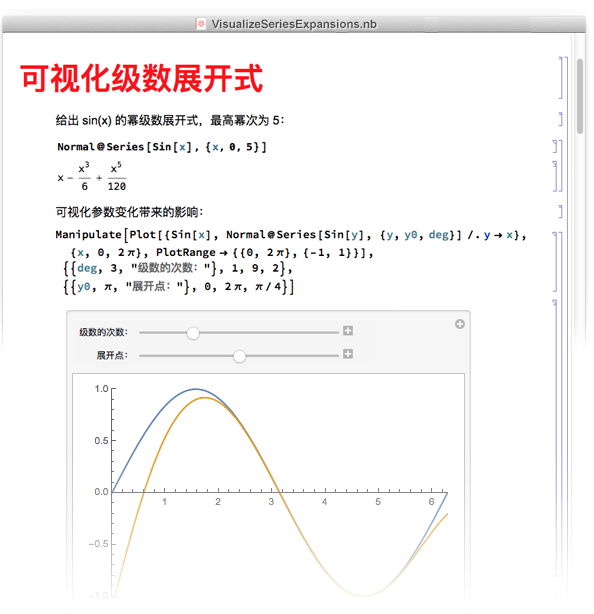
通过 Manipulate 命令可以交互式地实时查看改变参数会发生什么: In[1]:= Manipulate[Plot[Sin[f x], {x, -3, 3}, Filling -> Axis], {f, 1, 5}]
Out[1]= Manipulate[Plot[Sin[f x], {x, -3, 3}, Filling -> Axis], {f, 1, 5}]
Out[1]=
一个单独的 Manipulate 命令中可以有多个控件,Wolfram 语言将自动选择控件最合适的布局: In[1]:= Manipulate[Plot[Sin[f*x + p], {x, -3, 3}, Filling -> fill, PlotStyle -> color], {f, 1, 5}, {p, 3, 9}, {fill, {Bottom, Top, Axis}}, {color, Red}]
Out[1]= Manipulate[Plot[Sin[f*x + p], {x, -3, 3}, Filling -> fill, PlotStyle -> color], {f, 1, 5}, {p, 3, 9}, {fill, {Bottom, Top, Axis}}, {color, Red}]
Out[1]=
Wolfram 语言中的任意表达式都可被操控,包括非图形表达式: In[1]:= Manipulate[Expand[(a + b)^n], {n, 1, 20, 1}]
Out[1]= Manipulate[Expand[(a + b)^n], {n, 1, 20, 1}]
Out[1]=
 2.28 数学排版显示
用键盘快捷键(如 CTRL+/ 可用于分数的输入)插入可填充的排版表达式: (点击方框突出显示并填充,或按下 TAB 在各方框间移动.)
这是输入指数 (CTRL+6)、下标 (CTRL+-) 和其他常见表达式的简单方法. 在笔记本中按下 ESC 键得到 (在文档中常记为 ESC+alias+ESC )中. 键入正确的别名,当右侧的 (偏微分 “partial derivative” 的别名是 “pd”.)
产生求和、积分和其他高级表达式的方法为: (定积分 “definite integral” 的别名是 “dintt”.)
许多希腊字母和其他特殊字符也使用这种形式. 在桌面版的笔记本中,可以选择面板菜单中的“数学助手”查看可用的排版形式. 点击面板上的按钮即可在鼠标所在处插入一个可填充表达式:
使用 TraditionalForm 命令以传统数学符号显示任意表达式: In[1]:= TraditionalForm[(y + 3)^2/((y - 2) (y + 5))]
Out[1]= TraditionalForm[(y + 3)^2/((y - 2) (y + 5))]
Out[1]=

用 SHIFT+CMD+T (SHIFT+ALT+T)把现有单元转换成 TraditionalForm: (TraditionalForm 形式的表达式仍然是可计算的.) In[2]:= Limit[(x^2 - 1)/(x - 1), x -> 0]
In[3]:= Limit[(x^2 - 1)/(x - 1), x -> 0]
In[3]:=
 \!\(\*UnderscriptBox[\(lim\), \(x \[Rule] 0\)]\)( x^2 - 1)/(x - 1)
Out[3]= \!\(\*UnderscriptBox[\(lim\), \(x \[Rule] 0\)]\)( x^2 - 1)/(x - 1)
Out[3]=
 2.29 笔记本文档
可以在桌面或网页上使用 Wolfram 笔记本,它成功地把文字、图形、界面等与计算融合在一起:
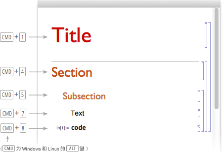
笔记本是按单元组织的,并由右边的方括号指定, 双击单元方括号打开或关闭单元组, 在单元间点击可以获取水平插入条,以便创建一个新的单元; 拷贝、粘贴、删除任何单元集合等. 选中任何单元集合并按住 SHIFT+ENTER 对输入进行计算. 在笔记本中可以加上标题、章节或文本单元:
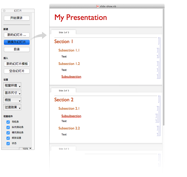
把笔记本转换成幻灯片也是易如反掌:
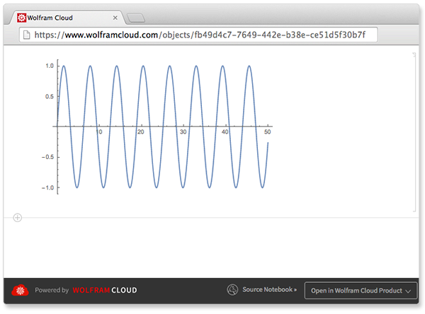
与 Wolfram 语言的其他内容一样,文档也是可被程序化改变的符号表达式. 2.30 云部署CloudDeploy 可把对象部署到 Wolfram Cloud. 创建一个有正弦波图片的网页: In[1]:= CloudDeploy[Plot[Sin[x], {x, 0, 50}]] CloudDeploy[Plot[Sin[x], {x, 0, 50}]]
[Out1]=
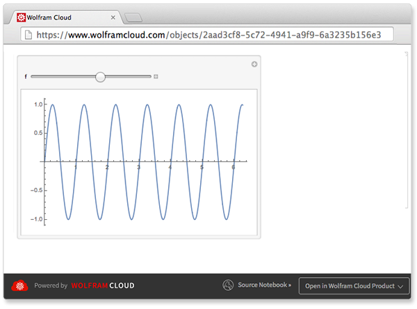
部署一个动态界面: In[1]:= CloudDeploy[Manipulate[Plot[Sin[f x], {x, 0, 2 Pi}], {f, 1, 10}]] CloudDeploy[Manipulate[Plot[Sin[f x], {x, 0, 2 Pi}], {f, 1, 10}]]
[Out1]=
无论是否是动态部署,从笔记本部署的内容都会保留其样式. 用 CloudDeploy[Delayed[...]] 部署表达式,每次被请求时都对其重新进行计算. 本文来自博客园,作者:ahrismile,转载请注明原文链接:https://www.cnblogs.com/ahrismile/p/15155772.html |


 .)
.) 表示为 I:
 符号.)
符号.)
 符号,可用在键盘快捷输入形式
 输入完成后,表达式就会发生改变:


【本文地址】