SOM自组织（竞争型）神经网络（Python实现）

2024-03-01 19:30| 来源: 网络整理| 查看: 265

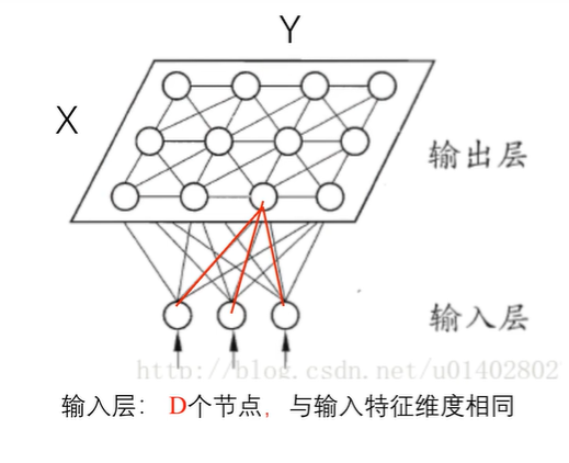
SOM是神经网络的一种，它可以将相互关系复杂且非线性的高维数据，映射到具有简单几何结构及相互关系的低维空间中进行展示。（低维映射能够反映高维特征之间的拓扑结构）

可以实现数据的可视化；聚类；分类；特征抽取等任务。（主要做数据可视化）

网络结构

相关解释

模型训练过程

具体细节

代码实现

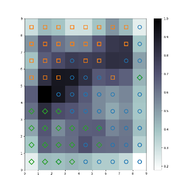
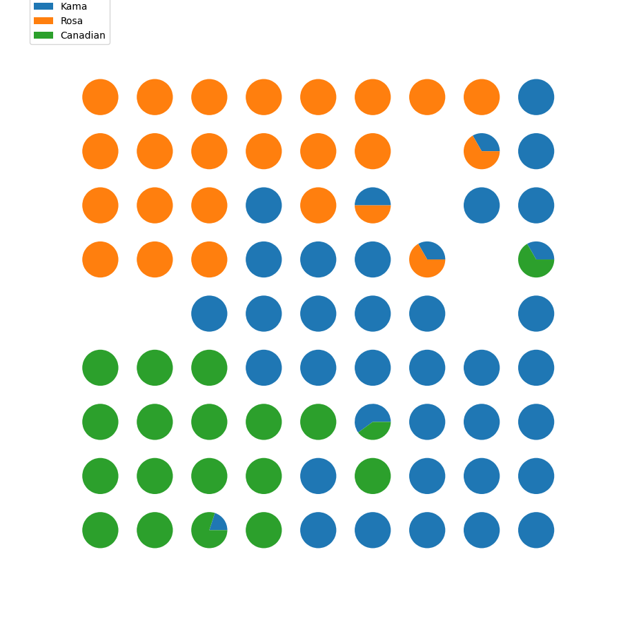
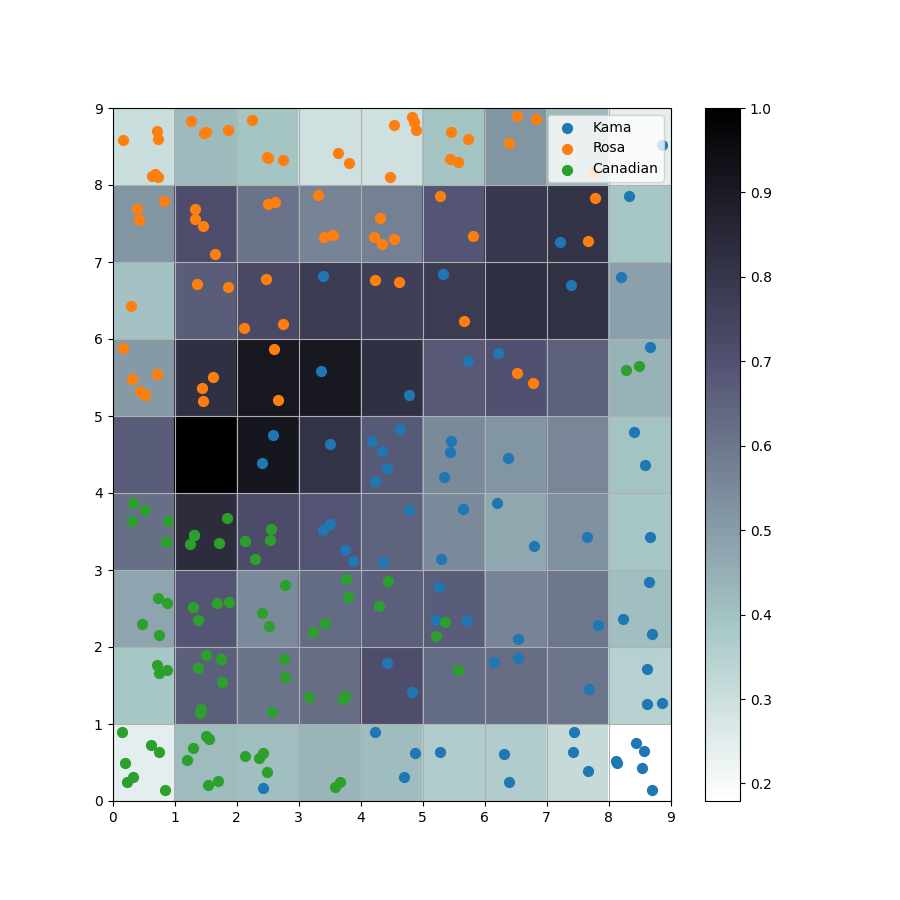
seeds_dataset数据集

链接: https://pan.baidu.com/s/1QYU70IGu8XEtHGDmm29KlA?pwd=yame 提取码: yame 复制这段内容后打开百度网盘手机App，操作更方便哦

训练模型 import numpy as np import random import tqdm import matplotlib.pyplot as plt import pandas as pd # 利用高斯距离法计算临近点的权重 # X,Y 模板大小，c 中心点的位置， sigma 影响半径 def gaussion_neighborhood(X, Y, c, sigma): xx, yy = np.meshgrid(np.arange(X), np.arange(Y)) d = 2 * sigma * sigma ax = np.exp(-np.power(xx - xx.T[c], 2) / d) ay = np.exp(-np.power(yy - yy.T[c], 2) / d) return (ax * ay).T # 利用bubble距离法计算临近点的权重 # X,Y 模板大小，c 中心点的位置， sigma 影响半径 def bubble_neighborhood(X, Y, c, sigma): neigx = np.arange(X) neigY = np.arange(Y) ax = np.logical_and(neigx > c[0] - sigma, neigx < c[0] + sigma) ay = np.logical_and(neigy > c[1] - sigma, neigy < c[1] + sigma) return np.outer(ax, ay) * 1. # 计算学习率 def get_learning_rate(lr, t, max_steps): return lr / (1 + t / (max_steps / 2)) # 计算欧式距离 def euclidean_distance(x, w): dis = np.expand_dims(x, axis=(0, 1)) - w return np.linalg.norm(dis, axis=-1) # 特征标准化 (x-mu)/std def feature_normalization(data): mu = np.mean(data, axis=0, keepdims=True) sigma = np.std(data, axis=0, keepdims=True) return (data - mu) / sigma # 获取激活节点的位置 def get_winner_index(x, w, dis_fun=euclidean_distance): # 计算输入样本和各个节点的距离 dis = dis_fun(x, w) # 找到距离最小的位置 index = np.where(dis == np.min(dis)) return (index[0][0], index[1][0]) def weights_PCA(X, Y, data): N, D = np.shape(data) weights = np.zeros([X, Y, D]) pc_length, pc = np.linalg.eig(np.cov(np.transpose(data))) pc_order = np.argsort(-pc_length) for i, c1 in enumerate(np.linspace(-1, 1, X)): for j, c2 in enumerate(np.linspace(-1, 1, Y)): weights[i, j] = c1 * pc[pc_order[0]] + c2 * pc[pc_order[1]] return weights # 计算量化误差 def get_quantization_error(datas, weights): w_x, w_y = zip(*[get_winner_index(d, weights) for d in datas]) error = datas - weights[w_x, w_y] error = np.linalg.norm(error, axis=-1) return np.mean(error) def train_SOM(X, Y, N_epoch, datas, init_lr=0.5, sigma=0.5, dis_fun=euclidean_distance, neighborhood_fun=gaussion_neighborhood, init_weight_fun=None, seed=20): # 获取输入特征的维度 N, D = np.shape(datas) # 训练的步数 N_steps = N_epoch * N # 对权重进行初始化 rng = np.random.RandomState(seed) if init_weight_fun is None: weights = rng.rand(X, Y, D) * 2 - 1 weights /= np.linalg.norm(weights, axis=-1, keepdims=True) else: weights = init_weight_fun(X, Y, datas) for n_epoch in range(N_epoch): print("Epoch %d" % (n_epoch + 1)) # 打乱次序 index = rng.permutation(np.arange(N)) for n_step, _id in enumerate(index): # 取一个样本 x = datas[_id] # 计算learning rate(eta) t = N * n_epoch + n_step eta = get_learning_rate(init_lr, t, N_steps) # 计算样本距离每个顶点的距离,并获得激活点的位置 winner = get_winner_index(x, weights, dis_fun) # 根据激活点的位置计算临近点的权重 new_sigma = get_learning_rate(sigma, t, N_steps) g = neighborhood_fun(X, Y, winner, new_sigma) g = g * eta # 进行权重的更新 weights = weights + np.expand_dims(g, -1) * (x - weights) # 打印量化误差 print("quantization_error= %.4f" % (get_quantization_error(datas, weights))) return weights def get_U_Matrix(weights): X, Y, D = np.shape(weights) um = np.nan * np.zeros((X, Y, 8)) # 8邻域 ii = [0, -1, -1, -1, 0, 1, 1, 1] jj = [-1, -1, 0, 1, 1, 1, 0, -1] for x in range(X): for y in range(Y): w_2 = weights[x, y] for k, (i, j) in enumerate(zip(ii, jj)): if (x + i >= 0 and x + i < X and y + j >= 0 and y + j < Y): w_1 = weights[x + i, y + j] um[x, y, k] = np.linalg.norm(w_1 - w_2) um = np.nansum(um, axis=2) return um / um.max() if __name__ == "__main__": # seed 数据展示 columns = ['area', 'perimeter', 'compactness', 'length_kernel', 'width_kernel', 'asymmetry_coefficient', 'length_kernel_groove', 'target'] data = pd.read_csv('seeds_dataset.txt', names=columns, sep='\t+', engine='python') labs = data['target'].values label_names = {1: 'Kama', 2: 'Rosa', 3: 'Canadian'} datas = data[data.columns[:-1]].values N, D = np.shape(datas) print(N, D) # 对训练数据进行正则化处理 datas = feature_normalization(datas) # SOM的训练 weights = train_SOM(X=9, Y=9, N_epoch=4, datas=datas, sigma=1.5, init_weight_fun=weights_PCA) # 获取UMAP UM = get_U_Matrix(weights) plt.figure(figsize=(9, 9)) plt.pcolor(UM.T, cmap='bone_r') # plotting the distance map as background plt.colorbar() markers = ['o', 's', 'D'] colors = ['C0', 'C1', 'C2'] for i in range(N): x = datas[i] w = get_winner_index(x, weights) i_lab = labs[i] - 1 plt.plot(w[0] + .5, w[1] + .5, markers[i_lab], markerfacecolor='None', markeredgecolor=colors[i_lab], markersize=12, markeredgewidth=2) plt.show()

结果图

SOM数据展示 import numpy as np import matplotlib.pyplot as plt import pandas as pd from SOM import train_SOM, feature_normalization, get_U_Matrix, get_winner_index, weights_PCA from collections import defaultdict, Counter import matplotlib.gridspec as gridspec if __name__ == "__main__": # seed 数据展示 columns = ['area', 'perimeter', 'compactness', 'length_kernel', 'width_kernel', 'asymmetry_coefficient', 'length_kernel_groove', 'target'] data = pd.read_csv('seeds_dataset.txt', names=columns, sep='\t+', engine='python') labs = data['target'].values label_names = {1: 'Kama', 2: 'Rosa', 3: 'Canadian'} datas = data[data.columns[:-1]].values N, D = np.shape(datas) print(N, D) # 对训练数据进行正则化处理 datas = feature_normalization(datas) # SOM的训练 X = 9 Y = 9 weights = train_SOM(X=X, Y=Y, N_epoch=4, datas=datas, sigma=1.5, init_weight_fun=weights_PCA) # 获取UMAP UM = get_U_Matrix(weights) print(UM) # '''画散点图''' # 显示UMAP plt.figure(1, figsize=(9, 9)) plt.pcolor(UM.T, cmap='bone_r') # plotting the distance map as background plt.colorbar() markers = ['o', 's', 'D'] colors = ['C0', 'C1', 'C2'] # 计算每个样本点投射后的坐标 w_x, w_y = zip(*[get_winner_index(d, weights) for d in datas]) w_x = np.array(w_x) w_y = np.array(w_y) # 分别把每一类的散点在响应的方格内进行打印（+随机位置偏移） for c in np.unique(labs): idx_target = (labs == c) plt.scatter(w_x[idx_target] + .5 + (np.random.rand(np.sum(idx_target)) - .5) * .8, w_y[idx_target] + .5 + (np.random.rand(np.sum(idx_target)) - .5) * .8, s=50, c=colors[c - 1], label=label_names[c]) plt.legend(loc='upper right') plt.grid() # plt.show() ''' 画饼图''' # 计算输出层的每个节点上映射了哪些数据 win_map = defaultdict(list) for x, lab in zip(datas, labs): win_map[get_winner_index(x, weights)].append(lab) # 统计每个输出节点上，映射了各类数据、各多少个 for pos in win_map: win_map[pos] = Counter(win_map[pos]) fig = plt.figure(2, figsize=(9, 9)) # 按照 X,Y对画面进行分格 the_grid = gridspec.GridSpec(Y, X, fig) print(the_grid) # 在每个格子里面画饼图 for pos in win_map.keys(): label_fracs = [win_map[pos][l] for l in label_names.keys()] plt.subplot(the_grid[Y - 1 - pos[1], pos[0]], aspect=1) patches, texts = plt.pie(label_fracs) plt.legend(labels=label_names.values(), loc='upper left', bbox_to_anchor=(-6, 10)) # plt.savefig('resulting_images/som_seed_pies.png') plt.show() 结果图

【本文地址】

公司简介

联系我们