| 如何在 Python 中绘制 ROC 曲线(一步一步) | 您所在的位置:网站首页 › python绘制auc曲线 › 如何在 Python 中绘制 ROC 曲线(一步一步) |
如何在 Python 中绘制 ROC 曲线(一步一步)
|
如何在 python 中绘制 roc 曲线(逐步)经过 本杰明·安德森博
7月 25, 2023
指导
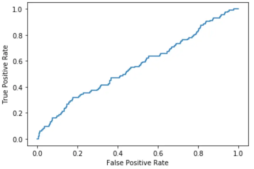
0 条评论 逻辑回归是一种统计方法,当响应变量是二元时,我们用它来拟合回归模型。为了评估逻辑回归模型对数据集的拟合程度,我们可以查看以下两个指标: 敏感性:当结果实际上是积极的时,模型预测观察结果为积极的概率。这也称为“真阳性率”。特异性:当结果实际上为负时,模型预测观察结果为负的概率。这也称为“真负率”。可视化这两个测量值的一种方法是创建ROC 曲线,它代表“接收器操作特性”曲线。该图显示逻辑回归模型的敏感性和特异性。 以下分步示例展示了如何在 Python 中创建和解释 ROC 曲线。 第1步:导入必要的包首先,我们将导入必要的包以在 Python 中执行逻辑回归: import pandas as pd import numpy as np from sklearn. model_selection import train_test_split from sklearn. linear_model import LogisticRegression from sklearn import metrics import matplotlib. pyplot as plt 步骤 2:拟合逻辑回归模型接下来,我们将导入一个数据集并对其拟合逻辑回归模型: #import dataset from CSV file on Github url = "https://raw.githubusercontent.com/Statorials/Python-Guides/main/default.csv" data = pd. read_csv (url) #define the predictor variables and the response variable X = data[[' student ',' balance ',' income ']] y = data[' default '] #split the dataset into training (70%) and testing (30%) sets X_train,X_test,y_train,y_test = train_test_split(X,y,test_size=0.3,random_state=0) #instantiate the model log_regression = LogisticRegression() #fit the model using the training data log_regression. fit (X_train,y_train)第三步:绘制ROC曲线接下来,我们将使用 Matplotlib 数据可视化包计算真阳性率和假阳性率并创建 ROC 曲线: #define metrics y_pred_proba = log_regression. predict_proba (X_test)[::,1] fpr, tpr, _ = metrics. roc_curve (y_test, y_pred_proba) #create ROC curve plt. plot (fpr,tpr) plt. ylabel (' True Positive Rate ') plt. xlabel (' False Positive Rate ') plt. show ()
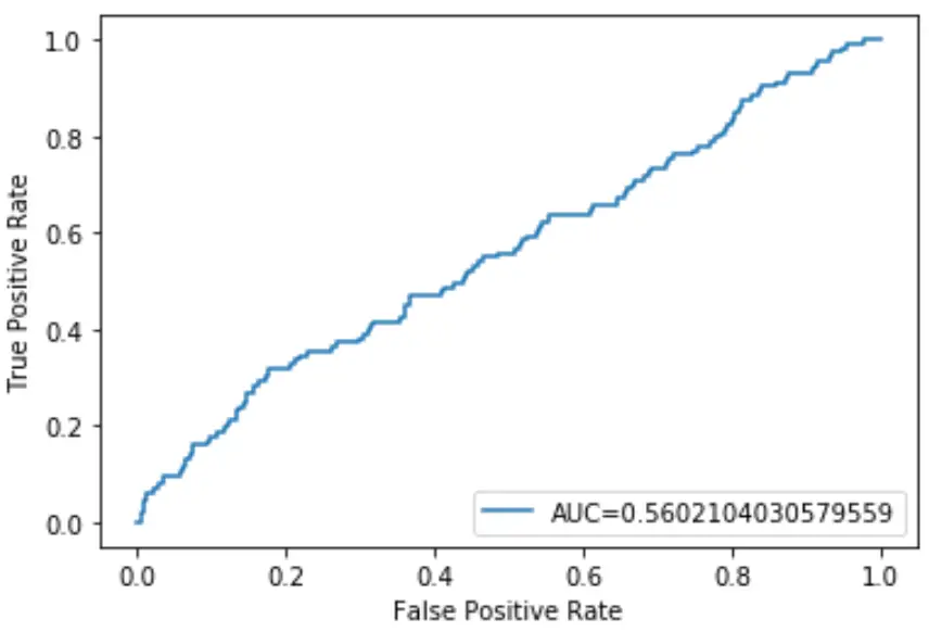
曲线越接近图的左上角,模型就越能够将数据分类。 从上图中我们可以看到,这个逻辑回归模型在将数据分类方面做得相当差。 为了量化这一点,我们可以计算 AUC(曲线下面积),它告诉我们有多少图位于曲线下。 AUC 越接近 1,模型越好。 AUC 等于 0.5 的模型并不比进行随机分类的模型更好。 第 4 步:计算 AUC我们可以使用以下代码来计算模型的AUC并将其显示在ROC图的右下角: #define metrics y_pred_proba = log_regression. predict_proba (X_test)[::,1] fpr, tpr, _ = metrics. roc_curve (y_test, y_pred_proba) auc = metrics. roc_auc_score (y_test, y_pred_proba) #create ROC curve plt. plot (fpr,tpr,label=" AUC= "+str(auc)) plt. ylabel (' True Positive Rate ') plt. xlabel (' False Positive Rate ') plt. legend (loc=4) plt. show ()
该逻辑回归模型的 AUC 为0.5602 。由于该数字接近 0.5,这证实该模型在数据分类方面做得很差。 相关:如何在 Python 中绘制多个 ROC 曲线 关于作者 本杰明·安德森博 本杰明·安德森博大家好,我是本杰明,一位退休的统计学教授,后来成为 Statorials 的热心教师。 凭借在统计领域的丰富经验和专业知识,我渴望分享我的知识,通过 Statorials 增强学生的能力。了解更多 添加评论取消回复 |
【本文地址】
公司简介
联系我们