| 位姿图优化(Ceres& G2O& GTSAM) | 您所在的位置:网站首页 › pi建节点有什么用 › 位姿图优化(Ceres& G2O& GTSAM) |
位姿图优化(Ceres& G2O& GTSAM)
位姿图优化(Ceres& G2O& GTSAM)
 敢敢のwings
分类:建图导航
个人专栏:从零到一的SLAM 发布时间 2023.02.22阅读数 216 评论数 0
0. 简介
敢敢のwings
分类:建图导航
个人专栏:从零到一的SLAM 发布时间 2023.02.22阅读数 216 评论数 0
0. 简介
作为SLAM中常用的方法,其原因是因为SLAM观测不只考虑到当前帧的情况,而需要加入之前状态量的观测。就比如一个在二维平面上移动的机器人,机器人可以使用一组传感器,例如车轮里程计或激光测距仪。从这些原始测量值中,我们想要估计机器人的轨迹并构建环境地图。为了降低问题的计算复杂度,位姿图方法将原始测量值抽象出来。具体来说,它创建了一个表示机器人姿态的节点图,以及表示两个节点之间的相对变换(增量位置和方向)的边。边缘是源自原始传感器测量值的虚拟测量值,例如通过集成原始车轮里程计或对齐从机器人获取的激光范围扫描。 之前作者已经已经在《SLAM本质剖析-Ceres》中详细的介绍了SLAM中对Ceres的使用。使用 Ceres Solver求解非线性优化问题,主要包括以下几部分: 构建代价函数(cost function)或残差(residual) 构建优化问题(ceres::Problem):通过 AddResidualBlock 添加代价函数(cost function)、损失函数(loss function核函数) 和 待优化状态量 配置求解器(ceres::Solver::Options) 运行求解器(ceres::Solve(options, &problem, &summary))与g2o优化中直接在边上添加information(信息矩阵)不同,Ceres无法直接实现此功能。 由于Ceres只接受最小二乘优化就,即$min(r^{^{T}}r)$;若要对残差加权,使用马氏距离即$min (r^{^{T}}\Sigma r)$,则要对信息矩阵(协方差矩阵)$\Sigma$做Cholesky分解:$LL^{^{T}}=\Sigma$,则$r^{^{T}}\Sigma r=r^{^{T}}(LL^{^{T}})r=(L^{^{T}}r)^{T}(L^{T}r)$,令$r’=L^{T}r$,最终得到纯种的最小二乘优化:$min(r’^{^{T}}r’)$。 1.2 Ceres优化步骤这一块的内容在前文中已经详细阐述了,这里就不详细分析了,下面直接贴一下每个部分的代码以及结构的组成。 Step1:构建Cost Function(1)AutoDiffCostFunction(自动求导) 构造 代价函数结构体或代价函数类(例如:struct CostFunctor),在其结构体内对模板括号() 重载用来定义残差; 在重载的 () 函数形参中,最后一个为残差,前面几个为待优化状态量,注意:形参类型必须是模板类型。 struct CostFunctor { template bool operator()(const T *const x, T *residual) const { residual[0] = 10.0 - x[0]; // r(x) = 10 - x return true; } }; 利用ceres::CostFunction *cost_function=new ceres::AutoDiffCostFunction(new costFunc),获得Cost Function模板参数分别是:代价结构体仿函数类型名,残差维度,第一个优化变量维度,第二个….;函数参数(new costFunc)是代价结构体(或类)对象,即此对象重载的 () 函数的函数指针 (2)NumericDiffCostFunction(数值求导) 数值求导法 也是构造 代价函数结构体,也需要重载括号()来定义残差,但在重载括号() 时没有用模板; struct CostFunctorNum { bool operator()(const double *const x, double *residual) const { residual[0] = 10.0 - x[0]; // r(x) = 10 - x return true; } }; 并且在实例化代价函数时也稍微有点区别,多了一个模板参数 ceres::CENTRAL ceres::CostFunction *cost_function; cost_function =new ceres::NumericDiffCostFunction(new CostFunctorNum);(3)自定义CostFunction 构建一个 继承自 ceres::SizedCostFunction 的类,同样,对于模板参数的数字,第一个为残差的维度,后面几个为待优化状态量的维度 ; 重载虚函数virtual bool Evaluate(double const* const* parameters, double *residuals, double **jacobians) const,根据 待优化变量,实现 残差和雅克比矩阵的计算(雅克比矩阵计算需要提供公式);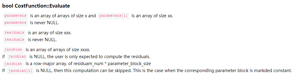 virtual bool Evaluate(double const* const* parameters, double* residuals, double** jacobians) const;:核心函数,跟自动求导中用仿函数中 operator() 类似,这里重写了基类中的 evaluate 函数,并且需要在其中定义误差和雅克比矩阵的计算方式:double const* const* parameters:参数块,主要是传入的各个节点,第一维度为节点的个数(这里是 6),第二维度则是对应节点的维度(这里两个节点的维度都是 6)double* residuals:残差,维度取决于误差的维度,这里是 6double** jacobians:雅克比矩阵,第一个维度为节点的个数(也就是要求解的雅克比矩阵的数量),第二个维度为对应雅克比矩阵的元素个数(这里两个雅克比矩阵的维度都是 6x6,因此维度是 36)详细的解析可以看一下这篇博客Ceres 学习记录(一):2D 位姿图优化```cpp virtual bool Evaluate(double const* const* parameters, double* residuals, double** jacobians) const;:核心函数,跟自动求导中用仿函数中 operator() 类似,这里重写了基类中的 evaluate 函数,并且需要在其中定义误差和雅克比矩阵的计算方式:double const* const* parameters:参数块,主要是传入的各个节点,第一维度为节点的个数(这里是 6),第二维度则是对应节点的维度(这里两个节点的维度都是 6)double* residuals:残差,维度取决于误差的维度,这里是 6double** jacobians:雅克比矩阵,第一个维度为节点的个数(也就是要求解的雅克比矩阵的数量),第二个维度为对应雅克比矩阵的元素个数(这里两个雅克比矩阵的维度都是 6x6,因此维度是 36)详细的解析可以看一下这篇博客Ceres 学习记录(一):2D 位姿图优化```cpp
class PoseGraphCFunc : public ceres::SizedCostFunction{public:EIGEN_MAKE_ALIGNED_OPERATOR_NEW;PoseGraphCFunc(const Sophus::SE3 measure,const Matrix6d covariance):_measure(measure),_covariance(covariance){}~PoseGraphCFunc(){}virtual bool Evaluate(double const_ const_ parameters,double _residuals,double **jacobians)const{//创建带有参数的SE3Sophus::SE3 pose_i=Sophus::SE3::exp(Vector6d(parameters[0]));//Eigen::MtatrixXd可以通过double指针来构造Sophus::SE3 pose_j=Sophus::SE3::exp(Vector6d(parameters[1]));Eigen::Map residual(residuals);//Eigen::Map(ptr)函数的作用是通过传入指针将c++数据映射为Eigen上的Matrix数据,有点与&相似//通过LLT分解得到信息矩阵residual=(_measure.inverse()_pose_i.inverse()_pose_j).log();Matrix6d sqrt_info=Eigen::LLT(_covariance).matrixLLT().transpose();//计算雅克比矩阵if(jacobians){if(jacobians[0]){Eigen::Map jacobian_i(jacobians[0]);Matrix6d Jr=JRInv(Sophus::SE3::exp(residual));jacobian_i=(sqrt_info)_(-Jr)_pose_j.inverse().Adj();}if(jacobians[1]){Eigen::Map jacobian_j(jacobians[1]);Matrix6d J = JRInv(Sophus::SE3::exp(residual));jacobian_j = sqrt_info _ J _ pose_j.inverse().Adj();}}residual=sqrt_info_residual;return true;second.x, &pose_end_iter->second.y, &pose_end_iter->second.yaw_radians); // 设置参数化,这里设置边的两个顶点的pose的旋转角度为 local_parameterization problem->SetParameterization(&pose_begin_iter->second.yaw_radians, angle_local_parameterization); problem->SetParameterization(&pose_end_iter->second.yaw_radians, angle_local_parameterization); } // The pose graph optimization problem has three DOFs that are not fully // constrained. This is typically referred to as gauge freedom. You can apply // a rigid body transformation to all the nodes and the optimization problem // will still have the exact same cost. The Levenberg-Marquardt algorithm has // internal damping which mitigate this issue, but it is better to properly // constrain the gauge freedom. This can be done by setting one of the poses // as constant so the optimizer cannot change it. std::map::iterator pose_start_iter = poses->begin(); CHECK(pose_start_iter != poses->end()) SetParameterBlockConstant(&pose_start_iter->second.x); problem->SetParameterBlockConstant(&pose_start_iter->second.y); problem->SetParameterBlockConstant(&pose_start_iter->second.yaw_radians); } 2. G2O的位姿图优化 G2O这部分也在我们的系列文章《SLAM本质剖析-G2O》中详细的阐述了。这里不详细的去写了。G2O本身就是经常被用于位姿图优化的,所以这里我们直接给出例子。算法的整个流程:1、构造g2o优化问题并执行优化;2、每次优化完成后,对地图点是否为外点进行卡方检验,检验到为内点的加入下次优化,否则下次不优化;3、得到优化后的当前帧的位姿(此函数只优化当前帧位姿) int Optimizer::PoseOptimization(Frame *pFrame) { // Step 1:这里先构造了大boss--g2o稀疏优化器, BlockSolver_6_3表示:位姿为6维,路标点是3维 g2o::SparseOptimizer optimizer;//图模型 g2o::BlockSolver_6_3::LinearSolverType * linearSolver;//线性求解器声明 // 创建一个线性求解器 linearSolver = new g2o::LinearSolverDense(); // 创建一个矩阵求解器并用上述线性求解器初始化 g2o::BlockSolver_6_3 * solver_ptr = new g2o::BlockSolver_6_3(linearSolver); //创建一个总的求解器,并用上述矩阵求解器初始化,可以看到这里使用了LM算法 g2o::OptimizationAlgorithmLevenberg* solver = new g2o::OptimizationAlgorithmLevenberg(solver_ptr); //设置求解器 optimizer.setAlgorithm(solver); // 输入的帧中,有效的,参与优化过程的2D-3D点对 int nInitialCorrespondences=0; // Step 2:添加顶点:待优化当前帧的位姿 g2o::VertexSE3Expmap * vSE3 = new g2o::VertexSE3Expmap();//创建一个顶点 vSE3->setEstimate(Converter::toSE3Quat(pFrame->mTcw));//转化成四元数+平移向量得形式 // 设置id vSE3->setId(0); // 要优化的变量,所以不能固定 vSE3->setFixed(false); optimizer.addVertex(vSE3);//添加顶点到优化器 // 地图点得个数,也就是要往优化器里添加得地图点个数。用于计算误差边(重投影误差) const int N = pFrame->N; vector vpEdgesMono; vector vpEdgesMono_FHR; vector vnIndexEdgeMono, vnIndexEdgeRight; vpEdgesMono.reserve(N); vpEdgesMono_FHR.reserve(N); vnIndexEdgeMono.reserve(N); vnIndexEdgeRight.reserve(N); vector vpEdgesStereo; vector vnIndexEdgeStereo; vpEdgesStereo.reserve(N); vnIndexEdgeStereo.reserve(N); // 下面涉及卡方分布去除外点的知识,这里不做讲解 // 自由度为2的卡方分布,显著性水平为0.05,对应的临界阈值5.991 const float deltaMono = sqrt(5.991); // 自由度为3的卡方分布,显著性水平为0.05,对应的临界阈值7.815 const float deltaStereo = sqrt(7.815); // Step 3:添加一元边(因为此函数只优化当前位姿) { // 锁定地图点。因为系统是多线程,所以在取数据时要加锁才能保证线程安全。 // 另一方面,需要使用地图点来构造顶点和边,因此不希望在构造的过程中部分地图点被改写造成不一致甚至是段错误 unique_lock lock(MapPoint::mGlobalMutex); // 遍历当前地图中的所有地图点 for(int i=0; imvpMapPoints[i]; // 如果这个地图点存在 if(pMP) { if(!pFrame->mpCamera2) { // 单目情况 if(pFrame->mvuRight[i]mvbOutlier[i] = false;// 先默认此地图点不是外点 // 对这个地图点的观测 Eigen::Matrix obs; const cv::KeyPoint &kpUn = pFrame->mvKeysUn[i]; obs setVertex(0, dynamic_cast(optimizer.vertex(0))); e->setMeasurement(obs);//设置测量值 // 这个点的置信度,其与特征点所在的图层有关。用信息矩阵(协方差矩阵得逆)来表示。 const float invSigma2 = pFrame->mvInvLevelSigma2[kpUn.octave]; e->setInformation(Eigen::Matrix2d::Identity()*invSigma2); // 在这里使用了鲁棒核函数 g2o::RobustKernelHuber* rk = new g2o::RobustKernelHuber; e->setRobustKernel(rk); rk->setDelta(deltaMono); // 设置相机内参 e->pCamera = pFrame->mpCamera; // 地图点的空间位置,作为迭代的初始值 cv::Mat Xw = pMP->GetWorldPos(); e->Xw[0] = Xw.at(0); e->Xw[1] = Xw.at(1); e->Xw[2] = Xw.at(2); optimizer.addEdge(e);//将此边加入优化器 vpEdgesMono.push_back(e);//记录边属于单目情况 vnIndexEdgeMono.push_back(i);//记录索引 } else // Stereo observation { nInitialCorrespondences++; pFrame->mvbOutlier[i] = false; // 观测多了一项右目的坐标 Eigen::Matrix obs; const cv::KeyPoint &kpUn = pFrame->mvKeysUn[i]; const float &kp_ur = pFrame->mvuRight[i]; obs setVertex(0, dynamic_cast(optimizer.vertex(0))); e->setMeasurement(obs); // 置信程度主要是看左目特征点所在的图层 const float invSigma2 = pFrame->mvInvLevelSigma2[kpUn.octave]; Eigen::Matrix3d Info = Eigen::Matrix3d::Identity()*invSigma2; e->setInformation(Info); g2o::RobustKernelHuber* rk = new g2o::RobustKernelHuber; e->setRobustKernel(rk); rk->setDelta(deltaStereo); //获得内参和地图点坐标作为初始值 e->fx = pFrame->fx; e->fy = pFrame->fy; e->cx = pFrame->cx; e->cy = pFrame->cy; e->bf = pFrame->mbf; cv::Mat Xw = pMP->GetWorldPos(); e->Xw[0] = Xw.at(0); e->Xw[1] = Xw.at(1); e->Xw[2] = Xw.at(2); optimizer.addEdge(e); vpEdgesStereo.push_back(e); vnIndexEdgeStereo.push_back(i); } } } } } // 如果没有足够的匹配点,那么就只好放弃了 //cout setLevel(1); // 设置为outlier , level 1 对应为外点,上面的过程中我们设置其为不优化 nBad++; } else { pFrame->mvbOutlier[idx]=false; e->setLevel(0); // 设置为inlier, level 0 对应为内点,上面的过程中我们就是要优化这些关系 } if(it==2) e->setRobustKernel(0); // 除了前两次优化需要RobustKernel以外, 其余的优化都不需要 -- 因为重投影的误差已经有明显的下降了 } // …… // Step 5 得到优化后的当前帧的位姿 g2o::VertexSE3Expmap* vSE3_recov = static_cast(optimizer.vertex(0)); g2o::SE3Quat SE3quat_recov = vSE3_recov->estimate(); cv::Mat pose = Converter::toCvMat(SE3quat_recov); pFrame->SetPose(pose);// 设置优化后得位姿 //cout points.size(), poseFrom.between(poseTo), odometryNoise)); initialEstimate.insert(cloudKeyPoses3D->points.size(), Pose3(Rot3::RzRyRx(transformAftMapped[2], transformAftMapped[0], transformAftMapped[1]),Point3(transformAftMapped[5], transformAftMapped[3], transformAftMapped[4]))); }6)更新isam和计算位姿 /*** update iSAM*/ isam->update(gtSAMgraph, initialEstimate); isam->update(); gtSAMgraph.resize(0); initialEstimate.clear(); /** save key poses*/ PointType thisPose3D; PointTypePose thisPose6D; Pose3 latestEstimate; isamCurrentEstimate = isam->calculateEstimate();//计算出最终矫正后结果存放的地方7)访问最终矫正后的位姿 int numPoses = isamCurrentEstimate.size(); for (int i = 0; i < numPoses; ++i) { cloudKeyPoses3D->points[i].x = isamCurrentEstimate.at(i).translation().y(); cloudKeyPoses3D->points[i].y = isamCurrentEstimate.at(i).translation().z(); cloudKeyPoses3D->points[i].z = isamCurrentEstimate.at(i).translation().x(); cloudKeyPoses6D->points[i].x = cloudKeyPoses3D->points[i].x; cloudKeyPoses6D->points[i].y = cloudKeyPoses3D->points[i].y; cloudKeyPoses6D->points[i].z = cloudKeyPoses3D->points[i].z; cloudKeyPoses6D->points[i].roll = isamCurrentEstimate.at(i).rotation().pitch(); cloudKeyPoses6D->points[i].pitch = isamCurrentEstimate.at(i).rotation().yaw(); cloudKeyPoses6D->points[i].yaw = isamCurrentEstimate.at(i).rotation().roll(); } 4. 参考链接https://blog.csdn.net/Curryfun/article/details/105894863https://blog.csdn.net/qq_42731705/article/details/120723600https://blog.csdn.net/ljtx200888/article/details/114278683https://xiaotaoguo.com/p/ceres-usage/https://blog.csdn.net/Walking_roll/article/details/119817174https://blog.csdn.net/lzy6041/article/details/107658568 图优化原创文章作者:敢敢のwings。如若转载,请注明出处:古月居 http://www.guyuehome.com/41992 打赏 0 点赞 0 收藏 0 分享 微信 微博 QQ 图片 上一篇:经典文献阅读之--VoxelMap(体素激光里程计) 下一篇:经典文献阅读之--DOGM(动态占用网格图) |
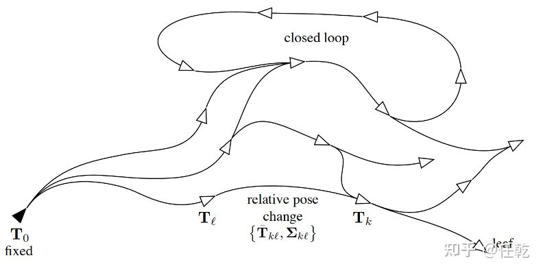 对上图的具体描述如下
【本文地址】