| 最全Python绘制多子图总结 | 您所在的位置:网站首页 › matlab绘制多个子图 › 最全Python绘制多子图总结 |
最全Python绘制多子图总结
|
实际操作中,想要在一个窗口(figure)的不同分区绘制多个子图 本文主要介绍最新的子图绘制中最有用的十三个功能,后续可补充。。。。 常用的是matplotlib.pyplot.subplot 格式:matplotlib.pyplot.subplot(*args,**kwargs) subplot(nrows, ncols, index, **kwargs) subplot(pos, **kwargs) subplot(**kwargs) subplot(ax)参数说明: *argsint, (int, int, index) 或 SubplotSpec,默认值:(1, 1, 1) 由以下之一描述的子图的位置: 1、三个整数(nrows、ncols、index)。子图将在具有 nrows 行和 ncols 列的网格上占据索引位置。索引从左上角的 1 开始,向右增加。 index 也可以是一个二元组,指定子图的(第一个,最后一个)索引 例如, fig.add_subplot(3, 1, (1, 2)) 制作一个跨越的子图图的上部 2/3。  2、一个 3 位整数。数字被解释为好像分别作为三个个位整数给出,即 fig.add_subplot(235) 与 fig.add_subplot(2, 3, 5) 相同。请注意,这只能在不超过 9 个子图的情况下使用 3、使用SubplotSpec,详细见十三 一、使用边距margins控制视图限制本示例中显示了如何使用边距代替 set_xlim 和 set_ylim 来放大和缩小绘图 import numpy as np import matplotlib.pyplot as plt from matplotlib.patches import Polygon def f(t): return np.exp(-t) * np.cos(2*np.pi*t) t1 = np.arange(0.0, 3.0, 0.01) ax1 = plt.subplot(212) ax1.margins(0.05) # Default margin is 0.05, value 0 means fit ax1.plot(t1, f(t1)) ax2 = plt.subplot(221) ax2.margins(2, 2) # Values >0.0 zoom out ax2.plot(t1, f(t1)) ax2.set_title('Zoomed out') ax3 = plt.subplot(222) ax3.margins(x=0, y=-0.25) # Values in (-0.5, 0.0) zooms in to center ax3.plot(t1, f(t1)) ax3.set_title('Zoomed in') plt.show()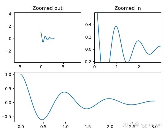 二、轴缩放效果from matplotlib.transforms import (
Bbox, TransformedBbox, blended_transform_factory)
from mpl_toolkits.axes_grid1.inset_locator import (
BboxPatch, BboxConnector, BboxConnectorPatch)
def connect_bbox(bbox1, bbox2,
loc1a, loc2a, loc1b, loc2b,
prop_lines, prop_patches=None):
if prop_patches is None:
prop_patches = {
**prop_lines,
"alpha": prop_lines.get("alpha", 1) * 0.2,
"clip_on": False,
}
c1 = BboxConnector(
bbox1, bbox2, loc1=loc1a, loc2=loc2a, clip_on=False, **prop_lines)
c2 = BboxConnector(
bbox1, bbox2, loc1=loc1b, loc2=loc2b, clip_on=False, **prop_lines)
bbox_patch1 = BboxPatch(bbox1, **prop_patches)
bbox_patch2 = BboxPatch(bbox2, **prop_patches)
p = BboxConnectorPatch(bbox1, bbox2,
# loc1a=3, loc2a=2, loc1b=4, loc2b=1,
loc1a=loc1a, loc2a=loc2a, loc1b=loc1b, loc2b=loc2b,
clip_on=False,
**prop_patches)
return c1, c2, bbox_patch1, bbox_patch2, p
def zoom_effect01(ax1, ax2, xmin, xmax, **kwargs):
"""
Connect *ax1* and *ax2*. The *xmin*-to-*xmax* range in both axes will
be marked.
Parameters
----------
ax1
The main axes.
ax2
The zoomed axes.
xmin, xmax
The limits of the colored area in both plot axes.
**kwargs
Arguments passed to the patch constructor.
"""
bbox = Bbox.from_extents(xmin, 0, xmax, 1)
mybbox1 = TransformedBbox(bbox, ax1.get_xaxis_transform())
mybbox2 = TransformedBbox(bbox, ax2.get_xaxis_transform())
prop_patches = {**kwargs, "ec": "none", "alpha": 0.2}
c1, c2, bbox_patch1, bbox_patch2, p = connect_bbox(
mybbox1, mybbox2,
loc1a=3, loc2a=2, loc1b=4, loc2b=1,
prop_lines=kwargs, prop_patches=prop_patches)
ax1.add_patch(bbox_patch1)
ax2.add_patch(bbox_patch2)
ax2.add_patch(c1)
ax2.add_patch(c2)
ax2.add_patch(p)
return c1, c2, bbox_patch1, bbox_patch2, p
def zoom_effect02(ax1, ax2, **kwargs):
"""
ax1 : the main axes
ax1 : the zoomed axes
Similar to zoom_effect01. The xmin & xmax will be taken from the
ax1.viewLim.
"""
tt = ax1.transScale + (ax1.transLimits + ax2.transAxes)
trans = blended_transform_factory(ax2.transData, tt)
mybbox1 = ax1.bbox
mybbox2 = TransformedBbox(ax1.viewLim, trans)
prop_patches = {**kwargs, "ec": "none", "alpha": 0.2}
c1, c2, bbox_patch1, bbox_patch2, p = connect_bbox(
mybbox1, mybbox2,
loc1a=3, loc2a=2, loc1b=4, loc2b=1,
prop_lines=kwargs, prop_patches=prop_patches)
ax1.add_patch(bbox_patch1)
ax2.add_patch(bbox_patch2)
ax2.add_patch(c1)
ax2.add_patch(c2)
ax2.add_patch(p)
return c1, c2, bbox_patch1, bbox_patch2, p
import matplotlib.pyplot as plt
plt.figure(figsize=(5, 5))
ax1 = plt.subplot(221)
ax2 = plt.subplot(212)
ax2.set_xlim(0, 1)
ax2.set_xlim(0, 5)
zoom_effect01(ax1, ax2, 0.2, 0.8)
ax1 = plt.subplot(222)
ax1.set_xlim(2, 3)
ax2.set_xlim(0, 5)
zoom_effect02(ax1, ax2)
plt.show() 二、轴缩放效果from matplotlib.transforms import (
Bbox, TransformedBbox, blended_transform_factory)
from mpl_toolkits.axes_grid1.inset_locator import (
BboxPatch, BboxConnector, BboxConnectorPatch)
def connect_bbox(bbox1, bbox2,
loc1a, loc2a, loc1b, loc2b,
prop_lines, prop_patches=None):
if prop_patches is None:
prop_patches = {
**prop_lines,
"alpha": prop_lines.get("alpha", 1) * 0.2,
"clip_on": False,
}
c1 = BboxConnector(
bbox1, bbox2, loc1=loc1a, loc2=loc2a, clip_on=False, **prop_lines)
c2 = BboxConnector(
bbox1, bbox2, loc1=loc1b, loc2=loc2b, clip_on=False, **prop_lines)
bbox_patch1 = BboxPatch(bbox1, **prop_patches)
bbox_patch2 = BboxPatch(bbox2, **prop_patches)
p = BboxConnectorPatch(bbox1, bbox2,
# loc1a=3, loc2a=2, loc1b=4, loc2b=1,
loc1a=loc1a, loc2a=loc2a, loc1b=loc1b, loc2b=loc2b,
clip_on=False,
**prop_patches)
return c1, c2, bbox_patch1, bbox_patch2, p
def zoom_effect01(ax1, ax2, xmin, xmax, **kwargs):
"""
Connect *ax1* and *ax2*. The *xmin*-to-*xmax* range in both axes will
be marked.
Parameters
----------
ax1
The main axes.
ax2
The zoomed axes.
xmin, xmax
The limits of the colored area in both plot axes.
**kwargs
Arguments passed to the patch constructor.
"""
bbox = Bbox.from_extents(xmin, 0, xmax, 1)
mybbox1 = TransformedBbox(bbox, ax1.get_xaxis_transform())
mybbox2 = TransformedBbox(bbox, ax2.get_xaxis_transform())
prop_patches = {**kwargs, "ec": "none", "alpha": 0.2}
c1, c2, bbox_patch1, bbox_patch2, p = connect_bbox(
mybbox1, mybbox2,
loc1a=3, loc2a=2, loc1b=4, loc2b=1,
prop_lines=kwargs, prop_patches=prop_patches)
ax1.add_patch(bbox_patch1)
ax2.add_patch(bbox_patch2)
ax2.add_patch(c1)
ax2.add_patch(c2)
ax2.add_patch(p)
return c1, c2, bbox_patch1, bbox_patch2, p
def zoom_effect02(ax1, ax2, **kwargs):
"""
ax1 : the main axes
ax1 : the zoomed axes
Similar to zoom_effect01. The xmin & xmax will be taken from the
ax1.viewLim.
"""
tt = ax1.transScale + (ax1.transLimits + ax2.transAxes)
trans = blended_transform_factory(ax2.transData, tt)
mybbox1 = ax1.bbox
mybbox2 = TransformedBbox(ax1.viewLim, trans)
prop_patches = {**kwargs, "ec": "none", "alpha": 0.2}
c1, c2, bbox_patch1, bbox_patch2, p = connect_bbox(
mybbox1, mybbox2,
loc1a=3, loc2a=2, loc1b=4, loc2b=1,
prop_lines=kwargs, prop_patches=prop_patches)
ax1.add_patch(bbox_patch1)
ax2.add_patch(bbox_patch2)
ax2.add_patch(c1)
ax2.add_patch(c2)
ax2.add_patch(p)
return c1, c2, bbox_patch1, bbox_patch2, p
import matplotlib.pyplot as plt
plt.figure(figsize=(5, 5))
ax1 = plt.subplot(221)
ax2 = plt.subplot(212)
ax2.set_xlim(0, 1)
ax2.set_xlim(0, 5)
zoom_effect01(ax1, ax2, 0.2, 0.8)
ax1 = plt.subplot(222)
ax1.set_xlim(2, 3)
ax2.set_xlim(0, 5)
zoom_effect02(ax1, ax2)
plt.show() 三、用紧凑的布局调整轴的大小tiny_layout 尝试调整图中子图的大小,以便轴对象和轴上的标签之间没有重叠。
import matplotlib.pyplot as plt
import itertools
import warnings
fontsizes = itertools.cycle([8, 16, 24, 32])
def example_plot(ax):
ax.plot([1, 2])
ax.set_xlabel('x-label', fontsize=next(fontsizes))
ax.set_ylabel('y-label', fontsize=next(fontsizes))
ax.set_title('Title', fontsize=next(fontsizes))
fig, ax = plt.subplots()
example_plot(ax)
plt.tight_layout() 三、用紧凑的布局调整轴的大小tiny_layout 尝试调整图中子图的大小,以便轴对象和轴上的标签之间没有重叠。
import matplotlib.pyplot as plt
import itertools
import warnings
fontsizes = itertools.cycle([8, 16, 24, 32])
def example_plot(ax):
ax.plot([1, 2])
ax.set_xlabel('x-label', fontsize=next(fontsizes))
ax.set_ylabel('y-label', fontsize=next(fontsizes))
ax.set_title('Title', fontsize=next(fontsizes))
fig, ax = plt.subplots()
example_plot(ax)
plt.tight_layout() fig, ((ax1, ax2), (ax3, ax4)) = plt.subplots(nrows=2, ncols=2)
example_plot(ax1)
example_plot(ax2)
example_plot(ax3)
example_plot(ax4)
plt.tight_layout() fig, ((ax1, ax2), (ax3, ax4)) = plt.subplots(nrows=2, ncols=2)
example_plot(ax1)
example_plot(ax2)
example_plot(ax3)
example_plot(ax4)
plt.tight_layout()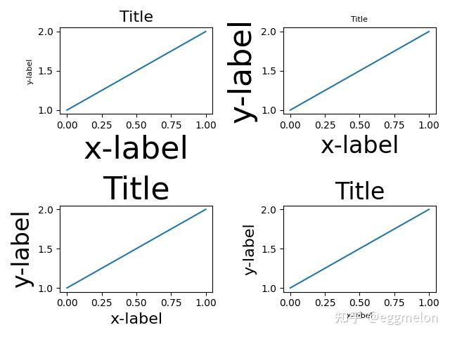 fig, (ax1, ax2) = plt.subplots(nrows=2, ncols=1)
example_plot(ax1)
example_plot(ax2)
plt.tight_layout() fig, (ax1, ax2) = plt.subplots(nrows=2, ncols=1)
example_plot(ax1)
example_plot(ax2)
plt.tight_layout() fig, (ax1, ax2) = plt.subplots(nrows=1, ncols=2)
example_plot(ax1)
example_plot(ax2)
plt.tight_layout() fig, (ax1, ax2) = plt.subplots(nrows=1, ncols=2)
example_plot(ax1)
example_plot(ax2)
plt.tight_layout() fig, axs = plt.subplots(nrows=3, ncols=3)
for ax in axs.flat:
example_plot(ax)
plt.tight_layout() fig, axs = plt.subplots(nrows=3, ncols=3)
for ax in axs.flat:
example_plot(ax)
plt.tight_layout()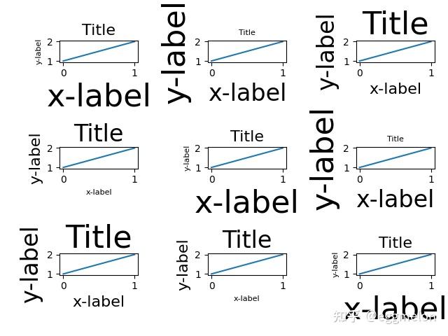 fig = plt.figure()
ax1 = plt.subplot(221)
ax2 = plt.subplot(223)
ax3 = plt.subplot(122)
example_plot(ax1)
example_plot(ax2)
example_plot(ax3)
plt.tight_layout() fig = plt.figure()
ax1 = plt.subplot(221)
ax2 = plt.subplot(223)
ax3 = plt.subplot(122)
example_plot(ax1)
example_plot(ax2)
example_plot(ax3)
plt.tight_layout() fig = plt.figure()
ax1 = plt.subplot2grid((3, 3), (0, 0))
ax2 = plt.subplot2grid((3, 3), (0, 1), colspan=2)
ax3 = plt.subplot2grid((3, 3), (1, 0), colspan=2, rowspan=2)
ax4 = plt.subplot2grid((3, 3), (1, 2), rowspan=2)
example_plot(ax1)
example_plot(ax2)
example_plot(ax3)
example_plot(ax4)
plt.tight_layout()
plt.show() fig = plt.figure()
gs1 = fig.add_gridspec(3, 1)
ax1 = fig.add_subplot(gs1[0])
ax2 = fig.add_subplot(gs1[1])
ax3 = fig.add_subplot(gs1[2])
example_plot(ax1)
example_plot(ax2)
example_plot(ax3)
gs1.tight_layout(fig, rect=[None, None, 0.45, None])
gs2 = fig.add_gridspec(2, 1)
ax4 = fig.add_subplot(gs2[0])
ax5 = fig.add_subplot(gs2[1])
example_plot(ax4)
example_plot(ax5)
with warnings.catch_warnings():
# gs2.tight_layout cannot handle the subplots from the first gridspec
# (gs1), so it will raise a warning. We are going to match the gridspecs
# manually so we can filter the warning away.
warnings.simplefilter("ignore", UserWarning)
gs2.tight_layout(fig, rect=[0.45, None, None, None])
# now match the top and bottom of two gridspecs.
top = min(gs1.top, gs2.top)
bottom = max(gs1.bottom, gs2.bottom)
gs1.update(top=top, bottom=bottom)
gs2.update(top=top, bottom=bottom)
plt.show() 四、地理投影 四、地理投影这显示了 4 种可能的地理预测。 Cartopy 支持更多的投影。 import matplotlib.pyplot as plt plt.figure() plt.subplot(projection="aitoff") plt.title("Aitoff") plt.grid(True) plt.figure()
plt.subplot(projection="hammer")
plt.title("Hammer")
plt.grid(True) plt.figure()
plt.subplot(projection="hammer")
plt.title("Hammer")
plt.grid(True) plt.figure()
plt.subplot(projection="lambert")
plt.title("Lambert")
plt.grid(True) plt.figure()
plt.subplot(projection="lambert")
plt.title("Lambert")
plt.grid(True) plt.figure()
plt.subplot(projection="mollweide")
plt.title("Mollweide")
plt.grid(True)
plt.show() plt.figure()
plt.subplot(projection="mollweide")
plt.title("Mollweide")
plt.grid(True)
plt.show() 五、共享轴限制和视图 五、共享轴限制和视图制作两个或更多共享一个轴的图是很常见的,例如,两个以时间为公共轴的子图。当您平移和缩放其中一个时,您希望另一个与您一起移动。为方便起见,matplotlib Axes 支持 sharex 和 sharey 属性。创建子图或轴时,您可以传入一个关键字,指示要与之共享的轴 import numpy as np import matplotlib.pyplot as plt t = np.arange(0, 10, 0.01) ax1 = plt.subplot(211) ax1.plot(t, np.sin(2*np.pi*t)) ax2 = plt.subplot(212, sharex=ax1) ax2.plot(t, np.sin(4*np.pi*t)) plt.show() 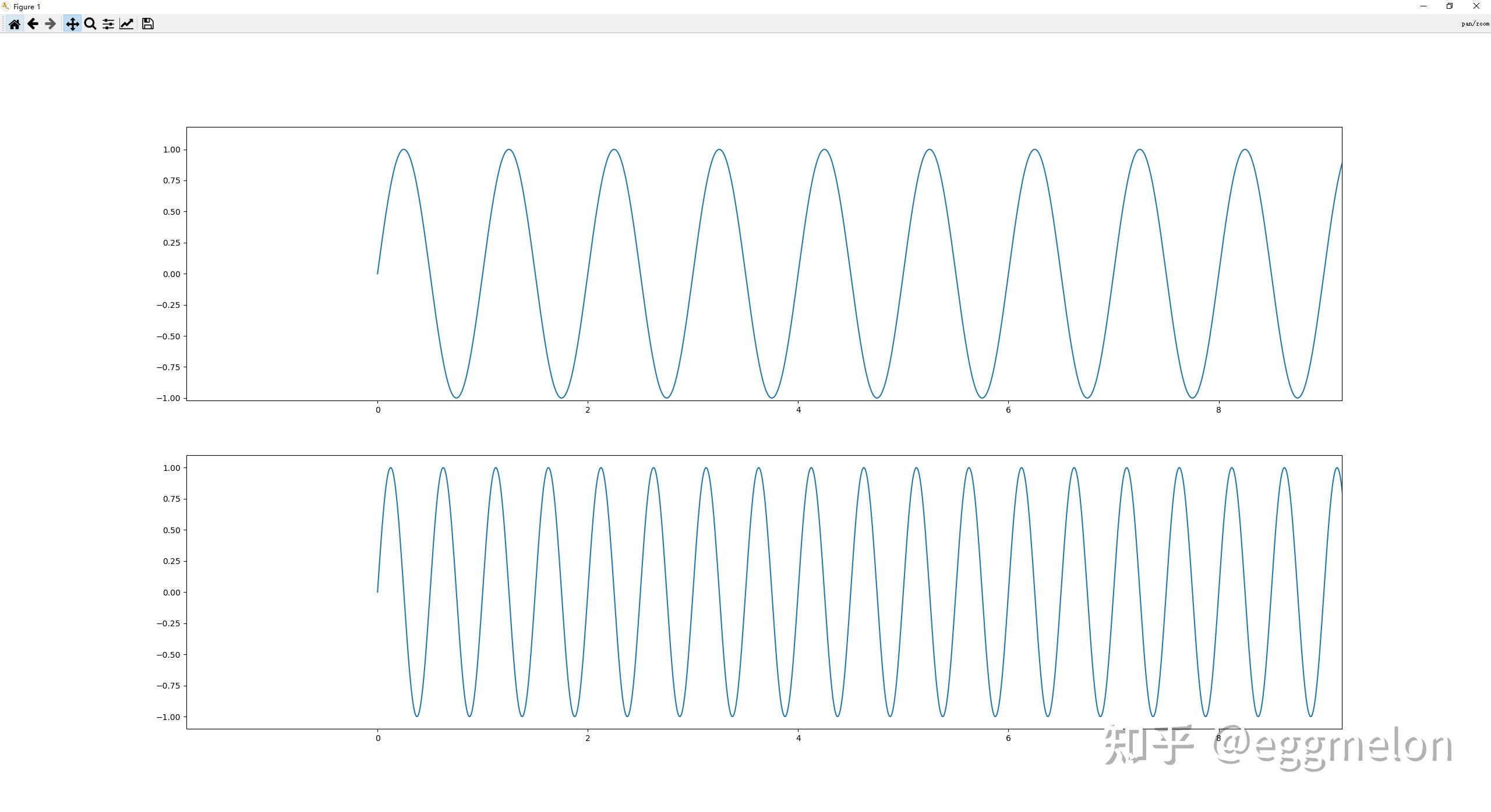 六、共享轴 六、共享轴通过将轴实例作为 sharex 或 sharey 关键字参数传递,您可以与另一个轴共享 x 或 y 轴限制。 更改一个轴上的轴限制将自动反映在另一个轴上,反之亦然,因此当您使用工具栏导航时,轴将在其共享轴上相互跟随。同样适用于轴缩放的变化(例如,对数与线性)。但是,刻度标签可能会有所不同,例如,您可以有选择地关闭一个轴上的刻度标签。 下面的示例显示了如何自定义各个轴上的刻度标签。共享轴共享刻度定位器、刻度格式器、视图限制和转换(例如,对数、线性)。但是刻度标签本身不共享属性。这是一个功能而不是错误,因为您可能希望使上轴上的刻度标签更小,例如,在下面的示例中。 import matplotlib.pyplot as plt import numpy as np t = np.arange(0.01, 5.0, 0.01) s1 = np.sin(2 * np.pi * t) s2 = np.exp(-t) s3 = np.sin(4 * np.pi * t) ax1 = plt.subplot(311) plt.plot(t, s1) plt.setp(ax1.get_xticklabels(), fontsize=6) # share x only ax2 = plt.subplot(312, sharex=ax1) plt.plot(t, s2) # make these tick labels invisible plt.setp(ax2.get_xticklabels(), visible=False) # share x and y ax3 = plt.subplot(313, sharex=ax1, sharey=ax1) plt.plot(t, s3) plt.xlim(0.01, 5.0) plt.show()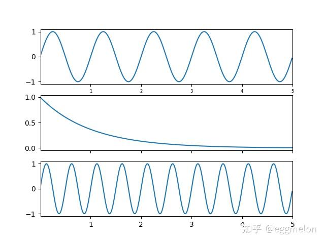 七、多个子图 七、多个子图带有多个子图的简单演示 import numpy as np import matplotlib.pyplot as plt x1 = np.linspace(0.0, 5.0) x2 = np.linspace(0.0, 2.0) y1 = np.cos(2 * np.pi * x1) * np.exp(-x1) y2 = np.cos(2 * np.pi * x2) fig, (ax1, ax2) = plt.subplots(2, 1) fig.suptitle('A tale of 2 subplots') ax1.plot(x1, y1, 'o-') ax1.set_ylabel('Damped oscillation') ax2.plot(x2, y2, '.-') ax2.set_xlabel('time (s)') ax2.set_ylabel('Undamped') plt.show()更加推荐第二种 x1 = np.linspace(0.0, 5.0) x2 = np.linspace(0.0, 2.0) y1 = np.cos(2 * np.pi * x1) * np.exp(-x1) y2 = np.cos(2 * np.pi * x2) plt.subplot(2, 1, 1) plt.plot(x1, y1, 'o-') plt.title('A tale of 2 subplots') plt.ylabel('Damped oscillation') plt.subplot(2, 1, 2) plt.plot(x2, y2, '.-') plt.xlabel('time (s)') plt.ylabel('Undamped') plt.show()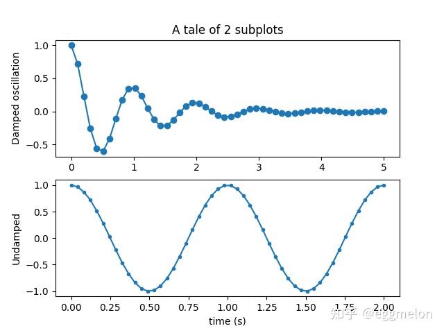 八、子图调整使用 subplots_adjust 调整边距和子图的间距
import matplotlib.pyplot as plt
import numpy as np
# Fixing random state for reproducibility
np.random.seed(19680801)
plt.subplot(211)
plt.imshow(np.random.random((100, 100)), cmap=plt.cm.BuPu_r)
plt.subplot(212)
plt.imshow(np.random.random((100, 100)), cmap=plt.cm.BuPu_r)
plt.subplots_adjust(bottom=0, right=0.8, top=1)#调整绘图区域的范围
cax = plt.axes([0.85, 0.1, 0.075, 0.8])
plt.colorbar(cax=cax)
plt.show() 八、子图调整使用 subplots_adjust 调整边距和子图的间距
import matplotlib.pyplot as plt
import numpy as np
# Fixing random state for reproducibility
np.random.seed(19680801)
plt.subplot(211)
plt.imshow(np.random.random((100, 100)), cmap=plt.cm.BuPu_r)
plt.subplot(212)
plt.imshow(np.random.random((100, 100)), cmap=plt.cm.BuPu_r)
plt.subplots_adjust(bottom=0, right=0.8, top=1)#调整绘图区域的范围
cax = plt.axes([0.85, 0.1, 0.075, 0.8])
plt.colorbar(cax=cax)
plt.show() 九、Pyplot 两个子图 九、Pyplot 两个子图使用 pyplot.subplot 创建一个带有两个子图的图 import numpy as np import matplotlib.pyplot as plt def f(t): return np.exp(-t) * np.cos(2*np.pi*t) t1 = np.arange(0.0, 5.0, 0.1) t2 = np.arange(0.0, 5.0, 0.02) plt.figure() plt.subplot(211) plt.plot(t1, f(t1), color='tab:blue', marker='o') plt.plot(t2, f(t2), color='black') plt.subplot(212) plt.plot(t2, np.cos(2*np.pi*t2), color='tab:orange', linestyle='--') plt.show()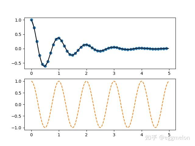 十、未链接的 MATPLOTLIB 十、未链接的 MATPLOTLIB来自脉冲星假信号的频率比较路径演示 import numpy as np import matplotlib.pyplot as plt import matplotlib.animation as animation # Fixing random state for reproducibility np.random.seed(19680801) # Create new Figure with black background fig = plt.figure(figsize=(8, 8), facecolor='black') # Add a subplot with no frame ax = plt.subplot(frameon=False) # Generate random data data = np.random.uniform(0, 1, (64, 75)) X = np.linspace(-1, 1, data.shape[-1]) G = 1.5 * np.exp(-4 * X ** 2) # Generate line plots lines = [] for i in range(len(data)): # Small reduction of the X extents to get a cheap perspective effect xscale = 1 - i / 200. # Same for linewidth (thicker strokes on bottom) lw = 1.5 - i / 100.0 line, = ax.plot(xscale * X, i + G * data[i], color="w", lw=lw) lines.append(line) # Set y limit (or first line is cropped because of thickness) ax.set_ylim(-1, 70) # No ticks ax.set_xticks([]) ax.set_yticks([]) # 2 part titles to get different font weights ax.text(0.5, 1.0, "MATPLOTLIB ", transform=ax.transAxes, ha="right", va="bottom", color="w", family="sans-serif", fontweight="light", fontsize=16) ax.text(0.5, 1.0, "UNCHAINED", transform=ax.transAxes, ha="left", va="bottom", color="w", family="sans-serif", fontweight="bold", fontsize=16) def update(*args): # Shift all data to the right data[:, 1:] = data[:, :-1] # Fill-in new values data[:, 0] = np.random.uniform(0, 1, len(data)) # Update data for i in range(len(data)): lines[i].set_ydata(i + G * data[i]) # Return modified artists return lines # Construct the animation, using the update function as the animation director. anim = animation.FuncAnimation(fig, update, interval=10) plt.show()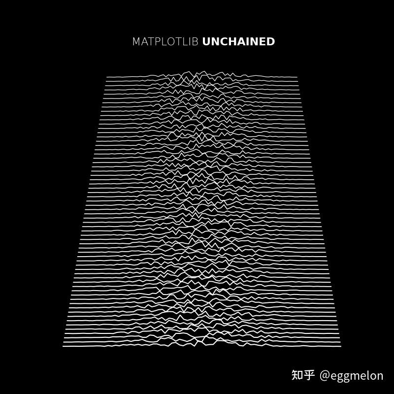 十一、严格的布局指南 十一、严格的布局指南如何使用紧凑布局在图形中干净地拟合绘图。 tiny_layout 自动调整子图参数,以便子图适合图形区域。这是一项实验性功能,可能不适用于某些情况。它只检查刻度标签、轴标签和标题的范围。 紧缩布局的替代方案是受约束的布局 简单示例 在 matplotlib 中,轴(包括子图)的位置在标准化图形坐标中指定。您的轴标签或标题(有时甚至是刻度标签)可能会超出图形区域,从而被剪裁 import matplotlib.pyplot as plt import numpy as np plt.rcParams['savefig.facecolor'] = "0.8" def example_plot(ax, fontsize=12): ax.plot([1, 2]) ax.locator_params(nbins=3) ax.set_xlabel('x-label', fontsize=fontsize) ax.set_ylabel('y-label', fontsize=fontsize) ax.set_title('Title', fontsize=fontsize) plt.close('all') fig, ax = plt.subplots() example_plot(ax, fontsize=24) 为了防止这种情况,需要调整轴的位置。对于子图,这可以通过调整子图参数来完成(移动轴的边缘为刻度标签腾出空间)。 Matplotlib v1.1 引入了自动为您执行此操作的 Figure.tight_layout。  fig, ax = plt.subplots()
example_plot(ax, fontsize=24)
plt.tight_layout() fig, ax = plt.subplots()
example_plot(ax, fontsize=24)
plt.tight_layout()请注意, matplotlib.pyplot.tight_layout() 只会在调用时调整子图参数。为了在每次重绘图形时执行此调整,您可以调用 fig.set_tight_layout(True),或者等效地将 rcParams["figure.autolayout"](默认值:False)设置为 True。 当您有多个子图时,您经常会看到不同轴的标签相互重叠 plt.close('all') fig, ((ax1, ax2), (ax3, ax4)) = plt.subplots(nrows=2, ncols=2) example_plot(ax1) example_plot(ax2) example_plot(ax3) example_plot(ax4) tiny_layout() 还将调整子图之间的间距以最小化重叠 fig, ((ax1, ax2), (ax3, ax4)) = plt.subplots(nrows=2, ncols=2) example_plot(ax1) example_plot(ax2) example_plot(ax3) example_plot(ax4) plt.tight_layout() tiny_layout() 可以采用 pad、w_pad 和 h_pad 的关键字参数。这些控制图形边框周围和子图之间的额外填充。焊盘以字体大小的分数指定。 fig, ((ax1, ax2), (ax3, ax4)) = plt.subplots(nrows=2, ncols=2) example_plot(ax1) example_plot(ax2) example_plot(ax3) example_plot(ax4) plt.tight_layout(pad=0.4, w_pad=0.5, h_pad=1.0) pad:float,默认值:1.08 图形边缘和子图边缘之间的填充,作为字体大小的一部分。 h_pad, w_pad:float, 默认值:pad 相邻子图边缘之间的填充(高度/宽度),作为字体大小的一部分。 rect:tuple (left, bottom, right, top), 默认: (0, 0, 1, 1) 标准化图形坐标中的矩形,整个子图区域(包括标签)将适合其中。  即使子图的大小不同,只要它们的网格规范兼容,tight_layout() 也能工作。在下面的示例中,ax1 和 ax2 是 2x2 网格的子图,而 ax3 是 1x2 网格的子图。 plt.close('all') fig = plt.figure() ax1 = plt.subplot(221) ax2 = plt.subplot(223) ax3 = plt.subplot(122) example_plot(ax1) example_plot(ax2) example_plot(ax3) plt.tight_layout()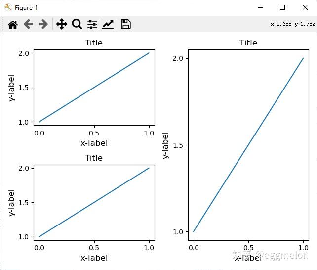 它适用于使用 subplot2grid() 创建的子图。通常,从 gridspec(使用 GridSpec 和其他函数自定义图形布局)创建的子图将起作用。 plt.close('all') fig = plt.figure() ax1 = plt.subplot2grid((3, 3), (0, 0)) ax2 = plt.subplot2grid((3, 3), (0, 1), colspan=2) ax3 = plt.subplot2grid((3, 3), (1, 0), colspan=2, rowspan=2) ax4 = plt.subplot2grid((3, 3), (1, 2), rowspan=2) example_plot(ax1) example_plot(ax2) example_plot(ax3) example_plot(ax4) plt.tight_layout()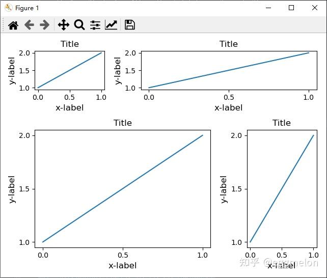 虽然没有经过彻底测试,但它似乎适用于带有 aspect != "auto" 的子图(例如,带有图像的轴) arr = np.arange(100).reshape((10, 10)) plt.close('all') fig = plt.figure(figsize=(5, 4)) ax = plt.subplot() im = ax.imshow(arr, interpolation="none") plt.tight_layout() 注意事项 默认情况下,tight_layout 会考虑轴上的所有artists。要从布局计算中删除artists,您可以调用 Artist.set_in_layout。 tiny_layout 假设artists所需的额外空间与轴的原始位置无关。这通常是正确的,但在极少数情况下并非如此。 pad=0 可以将一些文本裁剪几个像素。这可能是当前算法的错误或限制,目前尚不清楚为什么会发生这种情况。同时,建议使用大于 0.3 的焊盘。 与 GridSpec 一起使用 GridSpec 有自己的 GridSpec.tight_layout 方法(pyplot api pyplot.tight_layout 也有效)。 import matplotlib.gridspec as gridspec plt.close('all') fig = plt.figure() gs1 = gridspec.GridSpec(2, 1) ax1 = fig.add_subplot(gs1[0]) ax2 = fig.add_subplot(gs1[1]) example_plot(ax1) example_plot(ax2) gs1.tight_layout(fig)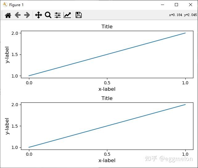 可以提供一个可选的 rect 参数,它指定子图将适合的边界框。坐标必须是标准化图形坐标,默认值为 (0, 0, 1, 1) fig = plt.figure() gs1 = gridspec.GridSpec(2, 1) ax1 = fig.add_subplot(gs1[0]) ax2 = fig.add_subplot(gs1[1]) example_plot(ax1) example_plot(ax2) gs1.tight_layout(fig, rect=[0, 0, 0.5, 1.0]) 但是,我们不建议使用它来手动构建更复杂的布局,例如在图的左侧有一个 GridSpec,在图的右侧有一个。对于这些用例,应改为利用嵌套网格规范或 Figure 子图 图例和注释 在 Matplotlib 2.2 之前,图例和注释被排除在决定布局的边界框计算之外。随后这些artists被添加到计算中,但有时不希望将他们包括在内。例如,在这种情况下,将轴缩小一点为图例腾出空间可能会很好: fig, ax = plt.subplots(figsize=(4, 3)) lines = ax.plot(range(10), label='A simple plot') ax.legend(bbox_to_anchor=(0.7, 0.5), loc='center left',) fig.tight_layout() plt.show() 然而,有时这是不希望的(在使用 fig.savefig('outname.png', bbox_inches='tight') 时很常见)。为了从边界框计算中删除图例,我们只需设置其边界 leg.set_in_layout(False) 并且图例将被忽略 fig, ax = plt.subplots(figsize=(4, 3)) lines = ax.plot(range(10), label='B simple plot') leg = ax.legend(bbox_to_anchor=(0.7, 0.5), loc='center left',) leg.set_in_layout(False) fig.tight_layout() plt.show()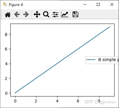 与 AxesGrid1 一起使用 虽然有限,但也支持 mpl_toolkits.axes_grid1 from mpl_toolkits.axes_grid1 import Grid plt.close('all') fig = plt.figure() grid = Grid(fig, rect=111, nrows_ncols=(2, 2), axes_pad=0.25, label_mode='L', ) for ax in grid: example_plot(ax) ax.title.set_visible(False) plt.tight_layout()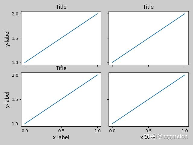 颜色条 如果您使用 Figure.colorbar 创建一个颜色条,则创建的颜色条将绘制在一个子图中,只要父轴也是一个子图,因此 Figure.tight_layout 将起作用 plt.close('all') arr = np.arange(100).reshape((10, 10)) fig = plt.figure(figsize=(4, 4)) im = plt.imshow(arr, interpolation="none") plt.colorbar(im) plt.tight_layout() 另一种选择是使用 AxesGrid1 工具包为颜色栏显式创建轴 from mpl_toolkits.axes_grid1 import make_axes_locatable plt.close('all') arr = np.arange(100).reshape((10, 10)) fig = plt.figure(figsize=(4, 4)) im = plt.imshow(arr, interpolation="none") divider = make_axes_locatable(plt.gca()) cax = divider.append_axes("right", "5%", pad="3%") plt.colorbar(im, cax=cax) plt.tight_layout() 十二、受限布局指南 十二、受限布局指南如何使用受约束的布局来干净地拟合图形中的绘图。 constrained_layout 自动调整子图和装饰,如图例和颜色条,使它们适合图形窗口,同时仍然尽可能地保留用户请求的逻辑布局。 受约束的布局类似于紧密布局,但使用约束求解器来确定允许它们适合的轴的大小。 在将任何轴添加到图形之前,需要激活 constrained_layout。这样做的两种方法是1、使用 subplots() 或 figure() 的相应参数 plt.subplots(constrained_layout=True) 2、通过 rcParams 激活它,例如: plt.rcParams['figure.constrained_layout.use'] = True 警告 目前约束布局是实验性的。行为和 API 可能会发生变化,或者整个功能可能会在没有弃用期的情况下被删除。如果您要求您的绘图绝对可重现,请在运行约束布局后获取轴位置,并在代码中使用 ax.set_position() 和 constrained_layout=False 简单示例 在 Matplotlib 中,轴(包括子图)的位置在标准化图形坐标中指定。您的轴标签或标题(有时甚至是刻度标签)可能会超出图形区域,从而被剪裁。 import matplotlib.pyplot as plt import matplotlib.colors as mcolors import matplotlib.gridspec as gridspec import numpy as np plt.rcParams['savefig.facecolor'] = "0.8" plt.rcParams['figure.figsize'] = 4.5, 4. plt.rcParams['figure.max_open_warning'] = 50 def example_plot(ax, fontsize=12, hide_labels=False): ax.plot([1, 2]) ax.locator_params(nbins=3) if hide_labels: ax.set_xticklabels([]) ax.set_yticklabels([]) else: ax.set_xlabel('x-label', fontsize=fontsize) ax.set_ylabel('y-label', fontsize=fontsize) ax.set_title('Title', fontsize=fontsize) fig, ax = plt.subplots(constrained_layout=False) example_plot(ax, fontsize=24) 为了防止这种情况,需要调整轴的位置。对于子图,这可以通过调整子图参数来完成(移动轴的边缘为刻度标签腾出空间)。但是,使用 constrained_layout=True kwarg 指定您的图形将自动进行调整  当您有多个子图时,您经常会看到不同轴的标签相互重叠 fig, axs = plt.subplots(2, 2, constrained_layout=False) for ax in axs.flat: example_plot(ax) 在对 plt.subplots 的调用中指定 constrained_layout=True 会导致布局被正确约束 fig, axs = plt.subplots(2, 2, constrained_layout=True) for ax in axs.flat: example_plot(ax)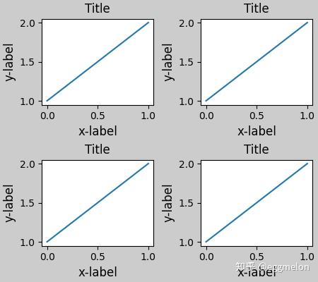 颜色条 如果您使用 Figure.colorbar 创建一个颜色条,则需要为它腾出空间。 constrained_layout 会自动执行此操作。请注意,如果您指定 use_gridspec=True 它将被忽略,因为此选项用于通过 tiny_layout 改进布局。 arr = np.arange(100).reshape((10, 10)) norm = mcolors.Normalize(vmin=0., vmax=100.) # see note above: this makes all pcolormesh calls consistent: pc_kwargs = {'rasterized': True, 'cmap': 'viridis', 'norm': norm} fig, ax = plt.subplots(figsize=(4, 4), constrained_layout=True) im = ax.pcolormesh(arr, **pc_kwargs) fig.colorbar(im, ax=ax, shrink=0.6) fig, axs = plt.subplots(2, 2, figsize=(4, 4), constrained_layout=True) for ax in axs.flat: im = ax.pcolormesh(arr, **pc_kwargs) fig.colorbar(im, ax=axs, shrink=0.6) 如果您为 colorbar 的 ax 参数指定轴列表(或其他可迭代容器),则 constrained_layout 将从指定轴中占用空间。 如果您从轴网格内指定轴列表,颜色条将适当地窃取空间并留下间隙,但所有子图仍将具有相同的大小 fig, axs = plt.subplots(3, 3, figsize=(4, 4), constrained_layout=True) for ax in axs.flat: im = ax.pcolormesh(arr, **pc_kwargs) fig.colorbar(im, ax=axs[1:, ][:, 1], shrink=0.8) fig.colorbar(im, ax=axs[:, -1], shrink=0.6) 字幕 constrained_layout 也可以为 suptitle 腾出空间 fig, axs = plt.subplots(2, 2, figsize=(4, 4), constrained_layout=True) for ax in axs.flat: im = ax.pcolormesh(arr, **pc_kwargs) fig.colorbar(im, ax=axs, shrink=0.6) fig.suptitle('Big Suptitle')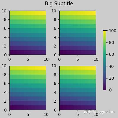 图例可以放置在其父轴之外。约束布局旨在为 Axes.legend() 处理此问题。但是,受约束的布局不处理通过 Figure.legend() (尚)创建的图例 填充和间距 轴之间的填充水平由 w_pad 和 wspace 控制,垂直由 h_pad 和 hspace 控制。这些可以通过 set_constrained_layout_pads 进行编辑。 w/h_pad 是以英寸为单位的轴周围的最小空间: fig, axs = plt.subplots(2, 2, constrained_layout=True) for ax in axs.flat: example_plot(ax, hide_labels=True) fig.set_constrained_layout_pads(w_pad=4 / 72, h_pad=4 / 72, hspace=0, wspace=0) 子图之间的间距由 wspace 和 hspace 进一步设置。这些被指定为整个子图组大小的一部分。如果这些值小于 w_pad 或 h_pad,则使用固定焊盘代替。请注意下面的边缘空间如何与上面的不同,但子图之间的空间会发生变化。 fig, axs = plt.subplots(2, 2, constrained_layout=True) for ax in axs.flat: example_plot(ax, hide_labels=True) fig.set_constrained_layout_pads(w_pad=4 / 72, h_pad=4 / 72, hspace=0.2, wspace=0.2) 如果多于两列,wspace是共享的,所以这里wspace被一分为二,每列之间的wspace为0.1 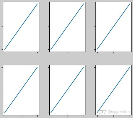 GridSpecs 也有可选的 hspace 和 wspace 关键字参数,它们将用于代替 constrained_layout 设置的 pads fig, axs = plt.subplots(2, 2, constrained_layout=True, gridspec_kw={'wspace': 0.3, 'hspace': 0.2}) for ax in axs.flat: example_plot(ax, hide_labels=True) # this has no effect because the space set in the gridspec trumps the # space set in constrained_layout. fig.set_constrained_layout_pads(w_pad=4 / 72, h_pad=4 / 72, hspace=0.0, wspace=0.0) plt.show() 颜色条间距 颜色条放置在距离其父级的距离垫上,其中垫是父级宽度的一小部分。然后由 w/hspace 给出到下一个子图的间距。 fig, axs = plt.subplots(2, 2, constrained_layout=True) pads = [0, 0.05, 0.1, 0.2] for pad, ax in zip(pads, axs.flat): pc = ax.pcolormesh(arr, **pc_kwargs) fig.colorbar(pc, ax=ax, shrink=0.6, pad=pad) ax.set_xticklabels('') ax.set_yticklabels('') ax.set_title(f'pad: {pad}') fig.set_constrained_layout_pads(w_pad=2 / 72, h_pad=2 / 72, hspace=0.2, wspace=0.2) 参数可以在脚本或 matplotlibrc 文件中设置五个 rcParams。它们都有前缀 figure.constrained_layout:use: 是否使用 constrained_layout。默认为假w_pad, h_pad:围绕轴对象填充。浮点数表示英寸。默认值为 3./72。英寸 (3 分)wspace, hspace:子图组之间的空间。浮点数表示被分隔的子图宽度的一小部分。默认值为 0.02。 plt.rcParams['figure.constrained_layout.use'] = True fig, axs = plt.subplots(2, 2, figsize=(3, 3)) for ax in axs.flat: example_plot(ax) 与 GridSpec 一起使用 受限布局旨在与 subplots() 或 GridSpec() 和 add_subplot() 一起使用。 请注意,在接下来的 constrained_layout=True 更复杂的 gridspec 布局是可能的。注意这里我们使用了方便的函数 add_gridspec 和 subgridspec。 fig = plt.figure() gs0 = fig.add_gridspec(1, 2) gs1 = gs0[0].subgridspec(2, 1) ax1 = fig.add_subplot(gs1[0]) ax2 = fig.add_subplot(gs1[1]) example_plot(ax1) example_plot(ax2) gs2 = gs0[1].subgridspec(3, 1) for ss in gs2: ax = fig.add_subplot(ss) example_plot(ax) ax.set_title("") ax.set_xlabel("") ax.set_xlabel("x-label", fontsize=12)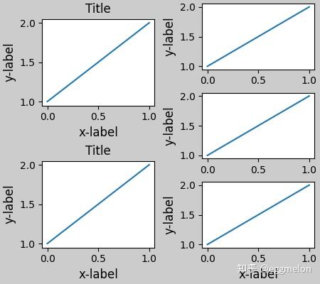 请注意,在上面的左列和右列没有相同的垂直范围。如果我们希望两个网格的顶部和底部对齐,那么它们需要在同一个 gridspec 中。我们还需要使这个数字更大,以便轴不会折叠到零高度: fig = plt.figure(figsize=(4, 6)) gs0 = fig.add_gridspec(6, 2) ax1 = fig.add_subplot(gs0[:3, 0]) ax2 = fig.add_subplot(gs0[3:, 0]) example_plot(ax1) example_plot(ax2) ax = fig.add_subplot(gs0[0:2, 1]) example_plot(ax, hide_labels=True) ax = fig.add_subplot(gs0[2:4, 1]) example_plot(ax, hide_labels=True) ax = fig.add_subplot(gs0[4:, 1]) example_plot(ax, hide_labels=True) fig.suptitle('Overlapping Gridspecs')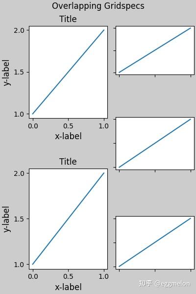 此示例使用两个 gridspecs 使颜色条仅与一组 pcolor 相关。请注意左栏比右两栏更宽的原因。当然,如果您希望子图的大小相同,您只需要一个 gridspec。 def docomplicated(suptitle=None): fig = plt.figure() gs0 = fig.add_gridspec(1, 2, figure=fig, width_ratios=[1., 2.]) gsl = gs0[0].subgridspec(2, 1) gsr = gs0[1].subgridspec(2, 2) for gs in gsl: ax = fig.add_subplot(gs) example_plot(ax) axs = [] for gs in gsr: ax = fig.add_subplot(gs) pcm = ax.pcolormesh(arr, **pc_kwargs) ax.set_xlabel('x-label') ax.set_ylabel('y-label') ax.set_title('title') axs += [ax] fig.colorbar(pcm, ax=axs) if suptitle is not None: fig.suptitle(suptitle) docomplicated()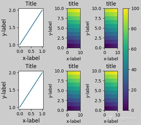 手动设置轴位置 手动设置轴位置可能有充分的理由。手动调用 set_position 将设置轴,因此 constrained_layout 不再对其产生影响。 (请注意, constrained_layout 仍然为移动的轴留下空间)。 fig, axs = plt.subplots(1, 2) example_plot(axs[0], fontsize=12) axs[1].set_position([0.2, 0.2, 0.4, 0.4]) 手动关闭 constrained_layout constrained_layout 通常会在每次绘制图形时调整轴位置。如果你想获得由 constrained_layout 提供的间距但没有更新,那么做初始绘制,然后调用 fig.set_constrained_layout(False)。这对于刻度标签可能改变长度的动画可能很有用。 请注意,对于使用工具栏的后端的 ZOOM 和 PAN GUI 事件,已关闭 constrained_layout。这可以防止轴在缩放和平移期间改变位置 限制 不兼容的功能 受限布局将与 pyplot.subplot 一起使用,但前提是每次调用的行数和列数都相同。原因是每次调用 pyplot.subplot 都会创建一个新的 GridSpec 实例,如果几何图形和 constrained_layout 不一样。所以以下工作正常: fig = plt.figure() ax1 = plt.subplot(2, 2, 1) ax2 = plt.subplot(2, 2, 3) # third axes that spans both rows in second column: ax3 = plt.subplot(2, 2, (2, 4)) example_plot(ax1) example_plot(ax2) example_plot(ax3) plt.suptitle('Homogenous nrows, ncols') 但以下会导致布局不佳: fig = plt.figure() ax1 = plt.subplot(2, 2, 1) ax2 = plt.subplot(2, 2, 3) ax3 = plt.subplot(1, 2, 2) example_plot(ax1) example_plot(ax2) example_plot(ax3) plt.suptitle('Mixed nrows, ncols') 类似地, subplot2grid 也有同样的限制,即 nrows 和 ncols 不能更改以使布局看起来不错 fig = plt.figure() ax1 = plt.subplot2grid((3, 3), (0, 0)) ax2 = plt.subplot2grid((3, 3), (0, 1), colspan=2) ax3 = plt.subplot2grid((3, 3), (1, 0), colspan=2, rowspan=2) ax4 = plt.subplot2grid((3, 3), (1, 2), rowspan=2) example_plot(ax1) example_plot(ax2) example_plot(ax3) example_plot(ax4) fig.suptitle('subplot2grid') 其他注意事项 constrained_layout 只考虑刻度标签、轴标签、标题和图例。因此,其他artists可能会被剪辑,也可能会重叠。 它假设刻度标签、轴标签和标题所需的额外空间与轴的原始位置无关。这通常是正确的,但在极少数情况下并非如此。 后端处理渲染字体的方式略有不同,因此结果不会是像素相同的。 使用超出轴边界的轴坐标的artists在添加到轴时会导致异常布局。这可以通过使用 add_artist() 将artists直接添加到图形来避免。有关示例,请参阅 ConnectionPatch。 调试 约束布局可能会以某种意想不到的方式失败。因为它使用约束求解器,所以求解器可以找到数学上正确的解决方案,但这根本不是用户想要的。通常的故障模式是所有尺寸都折叠到它们的最小允许值。如果发生这种情况,是由于以下两个原因之一: 没有足够的空间容纳您要求绘制的元素。 有一个错误 - 在这种情况下,请在 https://github.com/matplotlib/matplotlib/issues 上打开一个问题。 如果有错误,请使用不需要外部数据或依赖项(numpy 除外)的自包含示例报告。 十三、使用 GridSpec 和其他函数自定义图形布局如何创建网格状的轴组合 subplots() 也许是用于创建图形和轴的主要功能。它也与 matplotlib.pyplot.subplot() 类似,但会同时在图形上创建和放置所有轴。另见 matplotlib.figure.Figure.subplots GridSpec 指定将放置子图的网格的几何形状。需要设置网格的行数和列数。可选地,可以调整子图布局参数(例如,左、右等) SubplotSpec 指定子图在给定 GridSpec 中的位置 subplot2grid() 一个类似于 subplot() 的辅助函数,但使用基于 0 的索引并让 subplot 占据多个单元格。本教程不涉及此功能 import matplotlib.pyplot as plt import matplotlib.gridspec as gridspec基本快速入门指南前两个示例展示了如何使用 subplots() 和 gridspec 创建基本的 2×2 网格。使用 subplots() 非常简单。它返回一个 Figure 实例和一个 Axes 对象数组。 fig1, f1_axes = plt.subplots(ncols=2, nrows=2, constrained_layout=True)  对于像这样的简单用例,gridspec 可能过于冗长。您必须分别创建图形和 GridSpec 实例,然后将 gridspec 实例的元素传递给 add_subplot() 方法以创建轴对象。 gridspec 的元素通常以与 numpy 数组相同的方式访问 fig2 = plt.figure(constrained_layout=True) spec2 = gridspec.GridSpec(ncols=2, nrows=2, figure=fig2) f2_ax1 = fig2.add_subplot(spec2[0, 0]) f2_ax2 = fig2.add_subplot(spec2[0, 1]) f2_ax3 = fig2.add_subplot(spec2[1, 0]) f2_ax4 = fig2.add_subplot(spec2[1, 1])gridspec 的强大之处在于能够创建跨越行和列的子图。请注意用于选择每个子图将占用的 gridspec 部分的 NumPy 切片语法。请注意,我们还使用了方便的方法 Figure.add_gridspec 而不是 gridspec.GridSpec ,这可能会为用户节省导入,并保持命名空间清洁。 fig3 = plt.figure(constrained_layout=True) gs = fig3.add_gridspec(3, 3) f3_ax1 = fig3.add_subplot(gs[0, :]) f3_ax1.set_title('gs[0, :]') f3_ax2 = fig3.add_subplot(gs[1, :-1]) f3_ax2.set_title('gs[1, :-1]') f3_ax3 = fig3.add_subplot(gs[1:, -1]) f3_ax3.set_title('gs[1:, -1]') f3_ax4 = fig3.add_subplot(gs[-1, 0]) f3_ax4.set_title('gs[-1, 0]') f3_ax5 = fig3.add_subplot(gs[-1, -2]) f3_ax5.set_title('gs[-1, -2]') gridspec 对于通过几种方法创建不同宽度的子图也是必不可少的。 这里显示的方法类似于上面的方法,并初始化统一的网格规范,然后使用 numpy 索引和切片为给定的子图分配多个“单元格” fig4 = plt.figure(constrained_layout=True) spec4 = fig4.add_gridspec(ncols=2, nrows=2) anno_opts = dict(xy=(0.5, 0.5), xycoords='axes fraction', va='center', ha='center') f4_ax1 = fig4.add_subplot(spec4[0, 0]) f4_ax1.annotate('GridSpec[0, 0]', **anno_opts) fig4.add_subplot(spec4[0, 1]).annotate('GridSpec[0, 1:]', **anno_opts) fig4.add_subplot(spec4[1, 0]).annotate('GridSpec[1:, 0]', **anno_opts) fig4.add_subplot(spec4[1, 1]).annotate('GridSpec[1:, 1:]', **anno_opts) 另一种选择是使用 width_ratios 和 height_ratios 参数。这些关键字参数是数字列表。请注意,绝对值没有意义,只有它们的相对比率才重要。这意味着 width_ratios=[2, 4, 8] 等价于宽度相等的数字中的 width_ratios=[1, 2, 4] 。为了演示起见,我们将在 for 循环中盲目地创建轴,因为我们以后将不需要它们 fig5 = plt.figure(constrained_layout=True) widths = [2, 3, 1.5] heights = [1, 3, 2] spec5 = fig5.add_gridspec(ncols=3, nrows=3, width_ratios=widths, height_ratios=heights) for row in range(3): for col in range(3): ax = fig5.add_subplot(spec5[row, col]) label = 'Width: {}\nHeight: {}'.format(widths[col], heights[row]) ax.annotate(label, (0.1, 0.5), xycoords='axes fraction', va='center')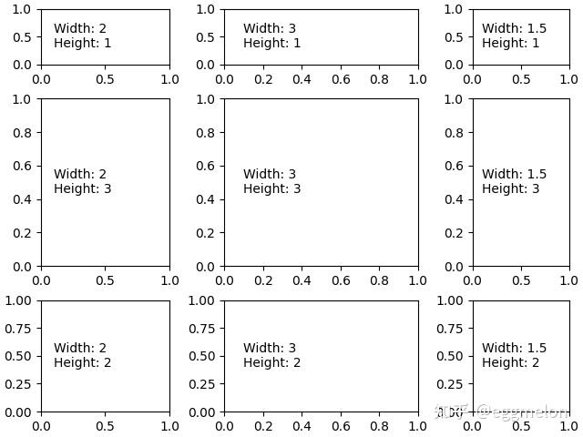 学习使用 width_ratios 和 height_ratios 特别有用,因为顶级函数 subplots() 在 gridspec_kw 参数中接受它们。就此而言,GridSpec 接受的任何参数都可以通过 gridspec_kw 参数传递给 subplots()。此示例在不直接使用 gridspec 实例的情况下重新创建了上一个图。 gs_kw = dict(width_ratios=widths, height_ratios=heights) fig6, f6_axes = plt.subplots(ncols=3, nrows=3, constrained_layout=True, gridspec_kw=gs_kw) for r, row in enumerate(f6_axes): for c, ax in enumerate(row): label = 'Width: {}\nHeight: {}'.format(widths[c], heights[r]) ax.annotate(label, (0.1, 0.5), xycoords='axes fraction', va='center')subplots 和 get_gridspec 方法可以组合使用,因为有时使用 subplots 制作大多数 subplots 然后删除一些并组合它们更方便。在这里,我们创建了一个布局,其中最后一列中的底部两个轴组合在一起。 fig7, f7_axs = plt.subplots(ncols=3, nrows=3) gs = f7_axs[1, 2].get_gridspec() # remove the underlying axes for ax in f7_axs[1:, -1]: ax.remove() axbig = fig7.add_subplot(gs[1:, -1]) axbig.annotate('Big Axes \nGridSpec[1:, -1]', (0.1, 0.5), xycoords='axes fraction', va='center') fig7.tight_layout() 对 Gridspec 布局的微调 当明确使用 GridSpec 时,您可以调整从 GridSpec 创建的子图的布局参数。请注意,此选项与 constrained_layout 或 Figure.tight_layout 不兼容,它们都调整子图大小以填充图形。 fig8 = plt.figure(constrained_layout=False) gs1 = fig8.add_gridspec(nrows=3, ncols=3, left=0.05, right=0.48, wspace=0.05) f8_ax1 = fig8.add_subplot(gs1[:-1, :]) f8_ax2 = fig8.add_subplot(gs1[-1, :-1]) f8_ax3 = fig8.add_subplot(gs1[-1, -1]) 这类似于 subplots_adjust(),但它只影响从给定 GridSpec 创建的子图。 比如比较这个图的左右两边: fig9 = plt.figure(constrained_layout=False) gs1 = fig9.add_gridspec(nrows=3, ncols=3, left=0.05, right=0.48, wspace=0.05) f9_ax1 = fig9.add_subplot(gs1[:-1, :]) f9_ax2 = fig9.add_subplot(gs1[-1, :-1]) f9_ax3 = fig9.add_subplot(gs1[-1, -1]) gs2 = fig9.add_gridspec(nrows=3, ncols=3, left=0.55, right=0.98, hspace=0.05) f9_ax4 = fig9.add_subplot(gs2[:, :-1]) f9_ax5 = fig9.add_subplot(gs2[:-1, -1]) f9_ax6 = fig9.add_subplot(gs2[-1, -1]) GridSpec 使用 SubplotSpec 您可以从 SubplotSpec 创建 GridSpec,在这种情况下,其布局参数设置为给定 SubplotSpec 的位置的布局参数。 请注意,这也可以从更详细的 gridspec.GridSpecFromSubplotSpec 中获得。 fig10 = plt.figure(constrained_layout=True) gs0 = fig10.add_gridspec(1, 2) gs00 = gs0[0].subgridspec(2, 3) gs01 = gs0[1].subgridspec(3, 2) for a in range(2): for b in range(3): fig10.add_subplot(gs00[a, b]) fig10.add_subplot(gs01[b, a]) 使用 SubplotSpec 的复杂嵌套 GridSpec 这是一个更复杂的嵌套 GridSpec 示例,我们通过在每个内部 3x3 网格中隐藏适当的脊椎,在外部 4x4 网格的每个单元周围放置一个框 import numpy as np def squiggle_xy(a, b, c, d, i=np.arange(0.0, 2*np.pi, 0.05)): return np.sin(i*a)*np.cos(i*b), np.sin(i*c)*np.cos(i*d) fig11 = plt.figure(figsize=(8, 8), constrained_layout=False) outer_grid = fig11.add_gridspec(4, 4, wspace=0, hspace=0) for a in range(4): for b in range(4): # gridspec inside gridspec inner_grid = outer_grid[a, b].subgridspec(3, 3, wspace=0, hspace=0) axs = inner_grid.subplots() # Create all subplots for the inner grid. for (c, d), ax in np.ndenumerate(axs): ax.plot(*squiggle_xy(a + 1, b + 1, c + 1, d + 1)) ax.set(xticks=[], yticks=[]) # show only the outside spines for ax in fig11.get_axes(): ss = ax.get_subplotspec() ax.spines.top.set_visible(ss.is_first_row()) ax.spines.bottom.set_visible(ss.is_last_row()) ax.spines.left.set_visible(ss.is_first_col()) ax.spines.right.set_visible(ss.is_last_col()) plt.show()
|
【本文地址】