matlab实现神经网络算法

2022-06-06 15:45| 来源: 网络整理| 查看: 265

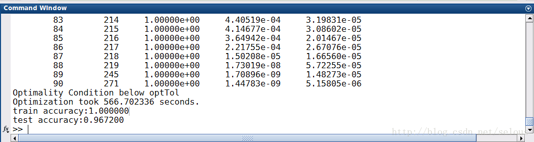
调试了两天，一边理解神经网络模型，一边在matlab上实现。刚刚终于调试通了minst手写体识别的简单神经网络。识别度不高，破机子也跑不起来太大规模的神经网络。就选了三层神经网络。

昨天晚上调通了之后只要隐含层的节点增大，就会偶尔出现过早拟合的问题。早上起来，把权值的初始化改小了之后，发现不会出现过早拟合的问题啦。当然这个参数初始化也是有讲究的，对于这个问题我也就采用了随意初始化。

当然不管是matlab还是python都有机器学习相关的包，但是如果想要深入理解神经网络模型的执行过程，我们还是需要自己手动实现的。当然关于数学优化的问题我是使用的ng之前提到过的minfunc函数。自己应该比较蛋疼。。。

初始化权值

initialWeight函数

function [stack] = initialWeight(H) %input: % H ，储存每层的节点个数 %output: % stack - 储存各层权值信息 %the number of layers; n = size(H,1); stack = cell(1,n-1); for i =1:n-1 stack{i}.w = rand(H(i+1),H(i))*0.001; stack{i}.b = zeros(H(i+1),1); end 列向量转化

param2stack

function [stack] = param2stack(param,H) % % Argument: % param - is the colume vector of all the weights and bias; % H - is the number of each layer unit except the bias unit % Output: % stack.w - is a cell data structure,and store the weights of all unit % except the bias unit.w{1} means the first layer weights. % stack.b - is a cell data structure,and store the weight of bias % unit. b{1} means the first weights of the first bias unit. % Functional: % transfer the colume weight vector to the cell data structure. %calculate the dimenstion of layer numbers. n = size(H,1); %initial the data struct; stack=cell(1,n-1); j=0; for i=1:n-1 stack{i}.b=param(j+1:j+H(i+1),1); j=j+H(i+1); stack{i}.w=reshape(param(j+1:j+H(i)*H(i+1)),[],H(i)); j=j+H(i)*H(i+1); end 参数矩阵转化为列向量

stack2param

function [param] = stack2param(stack,H) % % Argument: % H - is the number of each layer unit except the bias unit % param.w - is a cell data structure,and store the weights of all unit % except the bias unit.w{1} means the first layer weights. % param.b - is a cell data structure,and store the weight of bias % unit. b{1} means the first weights of the first bias unit. % Output: % a colume vector. % Functional: % transfer the colume weight vector to the cell data structure. %initial the cVector param = []; %calculate the dimenstion of layer numbers. n = size(H,1); for i=1:n-1 param = [param;stack{i}.b(:);stack{i}.w(:)]; % This can be optimized. But since our stacks are relatively short, it % is okay end 前向传播

forwardpropagation

function [a,z] = forwardpropagation(data,stack) %input: % data - is the set of samples;input value; % stack - is the weights of each layer. % stack{i}.w means the ith layer weight % stack{i}.b means the ith layer bais. %output: % a -is the the output of each layer all samples; % a{i} means the ith layer output. %the number of layers; n = size(stack,2)+1; %the number of samples; m = size(data,2); a = cell(1,n); z = cell(1,n); a{1} = data; for i=2:n z{i} = stack{i-1}.w*a{i-1}+repmat(stack{i-1}.b,[1,m]); a{i} = sigmoid(z{i}); end 损失函数

costFunction

function [f,g] = nero_regression(param, data,labels,ei) % % Arguments: % ei - the models information % % param - % % data - The examples stored in a matrix. % data(i,j) is the i'th coordinate of the j'th example. % labels - The label for each example. labels(j) is the j'th example's label. % %number of layers n = ei.layer_num; %number of samples; m = size(data,2); stack = param2stack(param,ei.layer_size); %forward propagation [a,z] = forwardpropagation(data,stack); %backward propagation delta = cell(1,n); y = zeros(size(a{n})); I = sub2ind(size(y), labels, 1:size(y,2)); y(I)=1; delta{n} = a{n} - y; for i =1:n-2 delta{n-i} = stack{n-i}.w'*delta{n-i+1}.*a{n-i}.*(1-a{n-i}); end %calculate the cost A = log(exp(z{n})./repmat(sum(exp(z{n})),[ei.layer_size(n),1])); f = -1/m*sum(A(I)); %regulazation %f = f + lamda * sum(param); %calculate the gradient gstack = cell(1,n-1); for i=1:n-1 %the dimension is H(i+1)*H(i); gstack{n-i}.w = (delta{n-i+1}*a{n-i}')/m + ei.lamda*stack{n-i}.w; gstack{n-i}.b = sum(delta{n-i+1},2)/m + ei.lamda*stack{n-i}.b; end g = stack2param(gstack,ei.layer_size); 主函数 addpath ../common addpath ../common/minFunc_2012/minFunc addpath ../common/minFunc_2012/minFunc/compiled addpath common % Load the MNIST data for this exercise. % train.X and test.X will contain the training and testing images. % Each matrix has size [n,m] where: % m is the number of examples. % n is the number of pixels in each image. % train.y and test.y will contain the corresponding labels (0 to 9). binary_digits = false; num_classes = 10; [train,test] = ex1_load_mnist(binary_digits); % Add row of 1s to the dataset to act as an intercept term. train.X = [ones(1,size(train.X,2)); train.X]; test.X = [ones(1,size(test.X,2)); test.X]; train.y = train.y+1; % make labels 1-based.%横向量 test.y = test.y+1; % make labels 1-based. % Training set info m=size(train.X,2); n=size(train.X,1); % Train softmax classifier using minFunc options=[]; options.display = 'iter'; options.maxFunEvals = 1e6; options.MaxIter = 200; %options.Method = 'lbfgs'; %the unit number of output layer output_num = 10; ei=[]; %define the ei.lamda = 0; %the dimension of input layer %the layer number of model ei.layer_num = 3; %the number unit of each layer ei.layer_size=[n;256;output_num]; stack = initialWeight(ei.layer_size); param = stack2param(stack,ei.layer_size); tic; % param=grad_check(@nero_regression, param, 5, train.X, train.y, ei); param=minFunc(@nero_regression, param, options, train.X, train.y, ei); fprintf('Optimization took %f seconds.\n', toc); % %theta=[theta, zeros(n,1)]; % expand theta to include the last class. % % % Print out training accuracy. tic; stack = param2stack(param,ei.layer_size); [a,~] = forwardpropagation(train.X,stack); [~,pred] = max(a{ei.layer_num}); acc_train = mean(pred==train.y); fprintf('train accuracy:%f\n',acc_train); % % % Print out test accuracy. [a,~]=forwardpropagation(test.X,stack); [~,pred] = max(a{ei.layer_num}); acc_test = mean(pred==test.y); fprintf('test accuracy:%f\n',acc_test);

最后的运行结果：

这里写图片描述

有点过拟合。。。调整一下lamda应该就可以了。

——2017.3.24

【本文地址】

公司简介

联系我们