4.4 matlab三维曲线（plot3函数、fplot3函数）

2023-12-18 14:20| 来源: 网络整理| 查看: 265

在这里插入图片描述

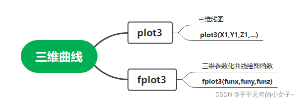
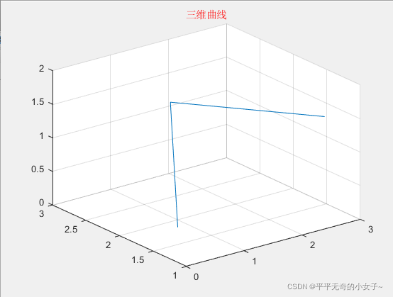
1、plot3函数 ( 1 ) plot3函数的基本用法 plot3(x，y，z) 其中，参数x、y、z组成一组曲线的坐标。

例1：绘制一条空间折线。

x = [0.2 1.8 2.5]; y = [1.3 2.8 1.1]; z = [0.4 1.2 1.6]; plot3(x,y,z) title('三维曲线','color','r') grid on axis([0,3,1,3,0,2])

在这里插入图片描述

t = linspace(0,14*pi,200); x = sin(t)+t.*cos(t); y = cos(t)-t.*sin(t); z = t; subplot(1,2,1) plot3(x,y,z) %有200个数据点，曲线较光滑 grid on subplot(1,2,2) plot3(x(1:3:200),y(1:3:200),z(1:3:200)) %有67个数据点，曲线较粗糙 grid on % subplot(1,2,2) % t1 = linspace(0,14*pi,80); % x1 = sin(t1)+t1.*cos(t1); % y1 = cos(t1)-t1.*sin(t1); % z1 = t1; % plot3(x1,y1,z1) % grid on

在这里插入图片描述

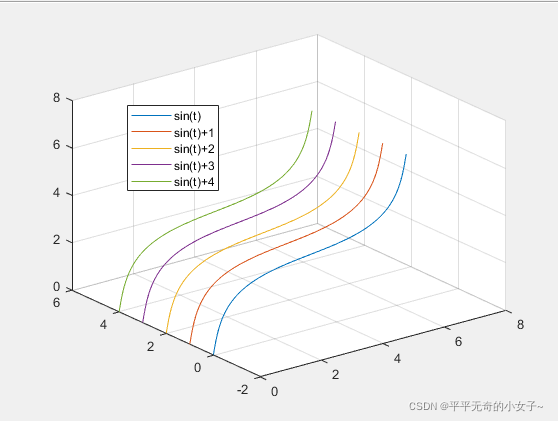
( 2 ) plot3函数参数的变化形式 plot3(x, y,z) ①参数x、y、z是同型矩阵：则以XYZ对应列元素绘制曲线，曲线条数等于短阵列数。 ②参数x、y、z中有向量，也有矩阵：向量的长度应与矩阵相符，行向量的长度与矩阵的列数相同，列向量的长度与矩阵的行数相同。

例3：在空间不同位置绘制5条正弦曲线。

方法1 列向量 t = linspace(0,2*pi,100); t = t'; x = [t t t t t]; y = [sin(t) sin(t)+1 sin(t)+2 sin(t)+3 sin(t)+4]; z = [t t t t t]; plot3(x,y,z) grid on legend('sin(t)','sin(t)+1','sin(t)+2','sin(t)+3','sin(t)+4','location','north') 方法2 行向量 t = linspace(0,2*pi,100); x = t; y = [sin(t);sin(t)+1;sin(t)+2;sin(t)+3;sin(t)+4]; z = t; plot3(x,y,z) grid on legend('sin(t)','sin(t)+1','sin(t)+2','sin(t)+3','sin(t)+4','location','north')

在这里插入图片描述 (3)含多组输入参数的plot3函数 plot3(x1, y1, z1,x2,y2,z2，…, xn, yn, zn) 每一组x、y、z向量构成一组数据点的坐标，绘制一条曲线。

例4：绘制三条不同长度的正弦曲线。

t1 = 0:0.01:1*pi; t2 = 0:0.01:2*pi; t3 = 0:0.01:3*pi; plot3(t1,sin(t1),t1,t2,sin(t2)+1,t2,t3,sin(t3)+2,t3) legend('sin(t1)','sin(t2)+1','sin(t3)+2','location','north') grid on

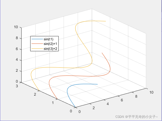在这里插入图片描述 (4)含选项的plot3函数 plot3(x, y,z,选项) 选项用于指定曲线的线型、颜色和数据点标记。

t = 0:pi/50:6*pi; x = cos(t); y = sin(t); z = 2*t; plot3(x,y,z,'p') %p以五角星输出 xlabel('X') ylabel('Y') zlabel('Z') grid on

在这里插入图片描述 2、fplot3函数 fplot3(funx, funy, funz, tlims) 其中, funx、funy、funz代表定义曲线x、y、z坐标的函数，通常采用函数句柄的形式。tlims为参数函数自变量的取值范围，用二元向量[tmin，tmax]描述﹐默认为[-5，5]。

xt = @(t)exp(-t/10).*sin(5*t); yt = @(t)exp(-t/10).*cos(5*t); zt = @(t)t; fplot3(xt,yt,zt,[-12,12],'b') xlabel('X') ylabel('Y') zlabel('Z') title('墨西哥冒顶曲线','fontsize',15,'color','r')

在这里插入图片描述

【本文地址】

公司简介

联系我们