| 非线性优化求解器(fminunc) | 您所在的位置:网站首页 › fminbnd函数用法 › 非线性优化求解器(fminunc) |
非线性优化求解器(fminunc)
|
优化工具包—无约束非线性优化求解器(fminunc)
原创不易,路过的各位大佬请点个赞 MATLAB基础代码/室内定位/导航/优化技术探讨:WX: ZB823618313 目录 优化工具包—无约束非线性优化求解器(fminunc)一、fminunc总体介绍二、fminunc求解器的具体用法三、举例:最小化多项式四、举例—获取最佳目标函数值五、检查求解过程(options 设置)六、信赖域法实例(fminunc求解器trust-region设置)6.1 信赖域实例16.2 信赖域实例2:使用问题结构体 fminunc函数:求无约束多变量函数的最小值
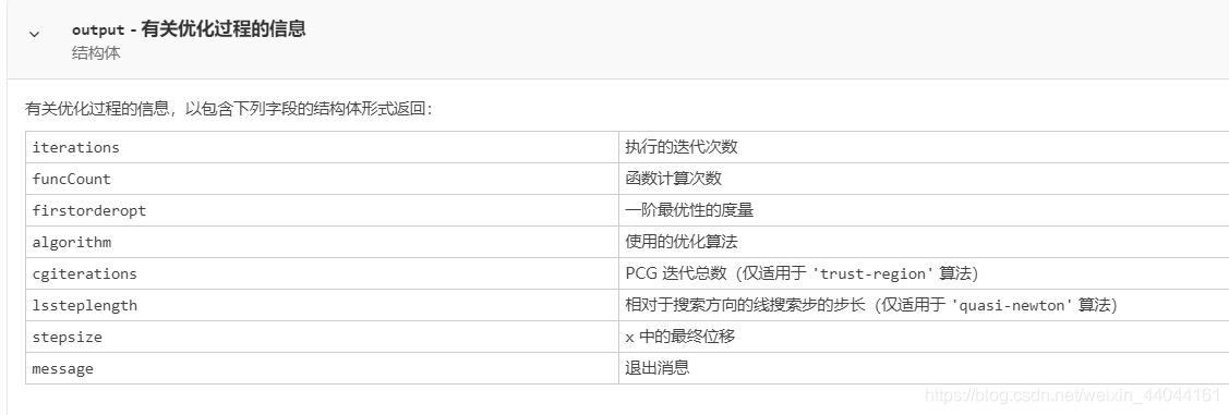
语法: x = fminunc(fun,x0) x = fminunc(fun,x0,options) x = fminunc(problem) [x,fval] = fminunc(___) [x,fval,exitflag,output] = fminunc(___) [x,fval,exitflag,output,grad,hessian] = fminunc(___)求解如下目标函数的最小值 min x f ( x ) \min_xf(x) xminf(x) 其中 f ( x ) f(x) f(x)目标损失函数,即优化函数。 x x x为变量,fminunc求解器面向多变量函数,因此 x x x可以是向量和矩阵。与fminbnd求解器不同,它的变量必须是单变量。此外,fminunc 适用于无约束非线性问题。如果需要优化的问题有约束,通常使用 fmincon。 x = fminunc(fun,x0) 在点 x0 处开始并尝试求 fun 中描述的函数的局部最小值 x。点 x0 可以是标量、向量或矩阵。 二、fminunc求解器的具体用法下面具体介绍fminunc求解器的用法 1)x = fminunc(fun,x0,options) 使用 options 中指定的优化选项最小化 fun。使用 optimoptions 可设置这些选项(后面介绍options); 2)x = fminunc(problem) 求 problem 的最小值,它是 problem 中所述的一个结构体,描述一个优化问题; 3)[x,fval] = fminunc(___) 对上述任何语法,返回目标函数 fun 在解 x 处的值; 4)[x,fval,exitflag,output] = fminunc(___) 还返回描述 fminunc 的退出条件的值 exitflag,以及提供优化过程信息的结构体 output。 5)[x,fval,exitflag,output,grad,hessian] = fminunc(___) 还返回: ~grad - fun 在解 x 处的梯度。 ~hessian - fun 在解 x 处的 Hessian 矩阵。请参阅 fminunc Hessian 矩阵。 目标函数: f ( x ) = 3 x 1 2 + 2 x 2 x 2 + x 2 2 − 4 x 1 + 5 x 2 f(x)=3x_1^2+2x_2x_2+x_2^2-4x_1+5x_2 f(x)=3x12+2x2x2+x22−4x1+5x2 其中 x = [ x 1 , x 2 ] x=[x_1,x_2] x=[x1,x2]为一个二维向量。 代码: 给定初始值x0=[1,1]; fun = @(x)3*x(1)^2 + 2*x(1)*x(2) + x(2)^2 - 4*x(1) + 5*x(2); x0 = [1,1]; [x,fval] = fminunc(fun,x0)求解结果:
当然也可以输出x处的梯度信息: fun = @(x) 3*x(1)^2 + 2*x(1)*x(2) + x(2)^2 - 4*x(1) + 5*x(2); x0 = [1,1]; [x,fval,exitflag,output,grad,hessian] = fminunc(fun,x0)
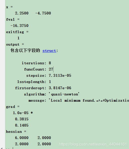
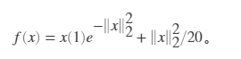
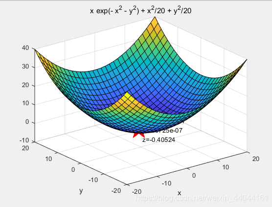
求非线性函数最小值的位置和该最小值处的函数值。目标函数是 结果如下 x = -0.6691 0.0000 fval = -0.4052 exitflag = 1 output = 包含以下字段的 struct: iterations: 9 funcCount: 42 stepsize: 2.9345e-04 lssteplength: 1 firstorderopt: 8.0839e-07 algorithm: ‘quasi-newton’ message: ‘Local minimum found.↵↵Optimization completed because the size of the gradient is less than↵the default value of the optimality tolerance.↵↵Stopping criteria details:↵↵Optimization completed: The first-order optimality measure, 6.891345e-07, is less ↵than options.OptimalityTolerance = 1.000000e-06.↵↵Optimization Metric Options↵relative norm(gradient) = 6.89e-07 OptimalityTolerance = 1e-06 (default)’ grad = 1.0e-06 * 0.8084 0.6817 hessian = 1.8998 -0.0000 -0.0000 0.9552 三维网格图如下: close all; fun = @(x)x(1)*exp(-(x(1)^2 + x(2)^2)) + (x(1)^2 + x(2)^2)/20; x0 = [1,2]; [x,fval,exitflag,output,grad,hessian] = fminunc(fun,x0) figure xmin=x(1);ymin=x(2);zmin=fval; syms x y z=x*exp(-(x^2 + y^2)) + (x^2 + y^2)/20; ezsurf(z,[-20,20],30);hold on; plot3(xmin,ymin,zmin,'rp','markersize',30,'MarkerFaceColor','r') %标记一个黑色的圆点 text(xmin,ymin,zmin,[' xmax=',num2str(xmin),char(10),' y=',num2str(ymin),char(10),' z=',num2str(zmin)]); %标出坐标
优化选项,指定为 optimoptions 的输出或 optimset 等返回的结构体。 语法: options = optimoptions(@fminunc,'Algorithm','quasi-newton');其中’Algorithm’设置优化工具包用什么优化算法求解问题,其中fminunc函数可以用拟牛顿法和信赖域算法。 设置fminunc采用拟牛顿法求解:其中该函数’Algorithm’的默认值为’quasi-newton’ options = optimoptions(@fminunc,'Algorithm','quasi-newton');quasi-newton 算法使用具有三次线搜索过程的 BFGS 拟牛顿法。这种拟牛顿法使用 BFGS公式来更新 Hessian 矩阵的逼近。您可以通过将 HessUpdate 选项设置为 ‘dfp’(并将 Algorithm 选项设置为 ‘quasi-newton’)来选择逼近逆 Hessian 矩阵的 DFP公式。您可以通过将 HessUpdate 设置为 ‘steepdesc’(并将 Algorithm 设置为 ‘quasi-newton’)来选择最陡下降法,尽管此设置通常效率不高。 设置fminunc采用信赖域算法求解:必须自己提供目标函数的梯度,不建议使用。 options = optimoptions(@fminunc,'Algorithm','trust-region');trust-region 算法要求您在 fun 中提供梯度,并使用 optimoptions 将 SpecifyObjectiveGradient 设置为 true。此算法是一种子空间信赖域方法,基于 [2] 和 [3] 中所述的内部反射牛顿法。每次迭代都涉及使用预条件共轭梯度法 (PCG) 来近似求解大型线性方程组。 用法: fun = @(x)x(1)*exp(-(x(1)^2 + x(2)^2)) + (x(1)^2 + x(2)^2)/20; x0 = [1,2]; [x,fval,exitflag,output,grad,hessian] = fminunc(fun,x0,options)其它options的参数表如下:
fminunc 有两种算法: ‘quasi-newton’(默认值) ‘trust-region’ 在命令行中使用 optimoptions 设置 Algorithm 选项。 建议 如果您的目标函数包括梯度,请使用 ‘Algorithm’ = ‘trust-region’,并将 SpecifyObjectiveGradient 选项设置为 true。 否则,请使用 ‘Algorithm’ = ‘quasi-newton’。 6.1 信赖域实例1考虑以下优化问题: 以下代码创建 rosenbrockwithgrad 函数,该函数包含梯度作为第二个输出。 function [f,g] = rosenbrockwithgrad(x) % Calculate objective f f = 100*(x(2) - x(1)^2)^2 + (1-x(1))^2; if nargout > 1 % gradient required g = [-400*(x(2)-x(1)^2)*x(1) - 2*(1-x(1)); 200*(x(2)-x(1)^2)]; end end创建使用目标函数的梯度的选项。此外,将算法设置为 ‘trust-region’。 options = optimoptions('fminunc','Algorithm','trust-region','SpecifyObjectiveGradient',true);将初始点设置为 [-1,2]。然后调用 fminunc。 x0 = [-1,2]; fun = @rosenbrockwithgrad; x = fminunc(fun,x0,options)结果 Local minimum found. Optimization completed because the size of the gradient is less than the value of the optimality tolerance. x = 1×2 1.0000 1.0000 6.2 信赖域实例2:使用问题结构体
将算法设置为 ‘trust-region’。 options = optimoptions('fminunc','Algorithm','trust-region','SpecifyObjectiveGradient',true);创建包括初始点 x0 = [-1,2] 的问题结构体。有关此结构体中的必填字段, problem.options = options; problem.x0 = [-1,2]; problem.objective = @rosenbrockwithgrad; problem.solver = 'fminunc';求解 x = fminunc(problem)结果 Local minimum found. Optimization completed because the size of the gradient is less than the value of the optimality tolerance. x = 1×2 1.0000 1.0000原创不易,路过的各位大佬请点个赞 |


 目标函数的三维网格图:
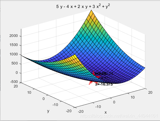
 画出等高线
画出等高线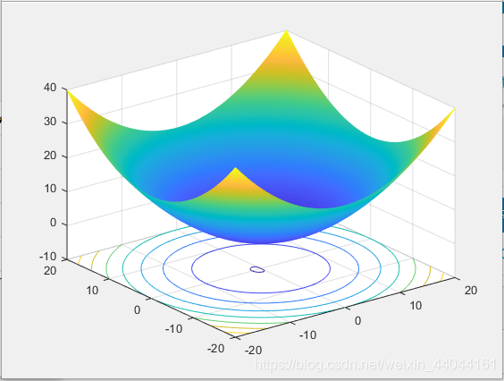

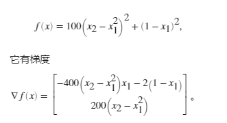
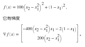 以下代码创建 rosenbrockwithgrad 函数,该函数包含梯度作为第二个输出。
【本文地址】