GAT原理+源码+dgl库快速实现 |
您所在的位置:网站首页 › 预测模型原理 › GAT原理+源码+dgl库快速实现 |
GAT原理+源码+dgl库快速实现
上次写了一个GCN的原理+源码+dgl实现brokenstring:GCN原理+源码+调用dgl库实现,这次按照上次的套路写写GAT的。GAT是图注意力神经网络的简写,其基本想法是给结点的邻居结点一个注意力权重,把邻居结点的信息聚合到结点上。 使用DGL库快速实现GAT这里以cora数据集为例,使用dgl库快速实现GAT模型进行图的结点分类问题。 import dgl import torch import torch.nn as nn import torch.nn.functional as F from dgl.nn.pytorch import GATConv from dgl import AddSelfLoop from dgl.data import CoraGraphDataset transform = ( AddSelfLoop() ) data = CoraGraphDataset(transform=transform) g = data[0] device = torch.device("cuda" if torch.cuda.is_available() else "cpu") g = g.int().to(device) features = g.ndata["feat"] labels = g.ndata["label"] masks = g.ndata["train_mask"], g.ndata["val_mask"], g.ndata["test_mask"] in_size = features.shape[1] out_size = data.num_classes print('*'*100) print(g) print('特征维度',features.shape) print('输出维度',len(torch.unique(labels))) print('边的条数',len(g.edges()[0])) print('边',g.edges()) class GAT(nn.Module): def __init__(self, in_feats, hidden_feats, out_feats, num_heads): super(GAT, self).__init__() self.num_heads = num_heads self.conv1 = GATConv(in_feats, hidden_feats, num_heads) self.conv2 = GATConv(hidden_feats*num_heads, out_feats, num_heads) self.dropout = nn.Dropout(0.5) def forward(self, g, x): h = self.conv1(g, x).flatten(1) h = F.elu(h) h = self.dropout(h) h = self.conv2(g, h).mean(1) return h def evaluate(g, features, labels, mask, model): model.eval() with torch.no_grad(): logits = model(g, features) logits = logits[mask] labels = labels[mask] #probabilities = F.softmax(logits, dim=1) #print(probabilities) _, indices = torch.max(logits, dim=1) correct = torch.sum(indices == labels) return correct.item() * 1.0 / len(labels) def train(g, features, labels, masks, model,epoches): # define train/val samples, loss function and optimizer train_mask = masks[0] val_mask = masks[1] loss_fcn = nn.CrossEntropyLoss() optimizer = torch.optim.Adam(model.parameters(), lr=1e-2, weight_decay=5e-4) # training loop for epoch in range(epoches): model.train() logits = model(g, features) loss = loss_fcn(logits[train_mask], labels[train_mask]) optimizer.zero_grad() loss.backward() optimizer.step() acc = evaluate(g, features, labels, val_mask, model) print( "Epoch {:05d} | Loss {:.4f} | Accuracy {:.4f} ".format( epoch, loss.item(), acc ) ) model = GAT(in_size, 4, out_size,num_heads=8).to(device) # model training print("Training...") epoches = 50 train(g, features, labels, masks, model,epoches) # test the model print("Testing...") acc = evaluate(g, features, labels, masks[2], model) print("Test accuracy {:.4f}".format(acc))上述代码可以直接运行,包括导数据、建模型、训练、预测一条龙服务。在这里,我们通过dgl库调用GATConv函数,注意到GATConv函数填入的参数有输入维度、输出维度、注意力头数,这样就可以很容易的建立起GAT层。接下来我们要进入源码探究下GATConv究竟是怎么构建的。 源码+原理这个部分,我将把源码和原理(公式)一一对应来分析GAT的构建机制。github源码见如下链接: https://github.com/gordicaleksa/pytorch-GAT 数据导入和预处理GAT源码中数据导入和预处理几乎和GCN的源码是一毛一样的,可以见brokenstring:GCN原理+源码+调用dgl库实现中的解读。唯一的区别就是GAT的源码把稀疏特征的归一化和邻接矩阵归一化分开了,如下图所示。其实,也不是那么有必要区分normalize_adj和normalize_features。因为度矩阵 D 为对角阵, D^{-\frac{1}{2}}AD^{-\frac{1}{2}}=D^{-1}A  GAT layer GAT layer我们先整体看下GAT layer的代码,代码在layers.py文件中 class GraphAttentionLayer(nn.Module): """ Simple GAT layer, similar to https://arxiv.org/abs/1710.10903 """ def __init__(self, in_features, out_features, dropout, alpha, concat=True): super(GraphAttentionLayer, self).__init__() self.dropout = dropout self.in_features = in_features self.out_features = out_features self.alpha = alpha self.concat = concat self.W = nn.Parameter(torch.empty(size=(in_features, out_features))) nn.init.xavier_uniform_(self.W.data, gain=1.414) self.a = nn.Parameter(torch.empty(size=(2*out_features, 1))) nn.init.xavier_uniform_(self.a.data, gain=1.414) self.leakyrelu = nn.LeakyReLU(self.alpha) def forward(self, h, adj): Wh = torch.mm(h, self.W) # h.shape: (N, in_features), Wh.shape: (N, out_features) e = self._prepare_attentional_mechanism_input(Wh) zero_vec = -9e15*torch.ones_like(e) attention = torch.where(adj > 0, e, zero_vec) attention = F.softmax(attention, dim=1) attention = F.dropout(attention, self.dropout, training=self.training) h_prime = torch.matmul(attention, Wh) if self.concat: return F.elu(h_prime) else: return h_prime def _prepare_attentional_mechanism_input(self, Wh): # Wh.shape (N, out_feature) # self.a.shape (2 * out_feature, 1) # Wh1&2.shape (N, 1) # e.shape (N, N) Wh1 = torch.matmul(Wh, self.a[:self.out_features, :]) Wh2 = torch.matmul(Wh, self.a[self.out_features:, :]) # broadcast add e = Wh1 + Wh2.T return self.leakyrelu(e) def __repr__(self): return self.__class__.__name__ + ' (' + str(self.in_features) + ' -> ' + str(self.out_features) + ')'接下来我们按照原论文慢慢拆解,原论文的链接如下https://arxiv.org/pdf/1710.10903.pdf 首先,我们定义结点的特征为  一共有 N 个结点,每个结点的特征都是F维的。这里的 h 就是forward函数输入的参数 h ,在cora数据集中 h 的维度2708*1433,即 N=2708 个结点和 F=1433 个结点特征。 第一步,我们需要对结点特征进行一个线性降维,即 W_h=hW , W\in R^{F\times F'} 。源码中 F'=8 即为GCN层输出神经元维度,在__init__里为参数output_features。上述操作对应forward函数里的 Wh = torch.mm(h, self.W) # h.shape: (N, in_features), Wh.shape: (N, out_features)第二步,注意力机制的生成。在源码里对应_prepare_attentional_mechanism_input函数。原论文中注意力系数定义为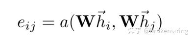 该式子表示 结点i对结点j 的注意力系数,其中 a 是一个函数:  可以把两个 F' 维的向量映射到实数上。论文中 a() 是用一个线性层来实现。记权重向量 \text{a}\in R^{ 2F'} , \text{a}=[\text{a}_1,\text{a}_2] , \text{a}_1,\text{a}_2\in R^{F'} 。这里有关向量 \text{a} 的定义在__init__函数中 self.a = nn.Parameter(torch.empty(size=(2*out_features, 1)))e_{ij}= a(Wh_i,Wh_j) = \text{a}^T[Wh_i,Wh_j]=\text{a}^TWh_i+\text{a}^TWh_j 该步运算在 _prepare_attentional_mechanism_input函数中计算。注意该函数计算了所有结点间的 e_{ij} 。为了防止梯度爆炸和梯度消失,作者最后还做了一层leakrelu,即e_{ij}=Leakrelu(e_{ij}) 。 def _prepare_attentional_mechanism_input(self, Wh): # Wh.shape (N, out_feature) # self.a.shape (2 * out_feature, 1) # Wh1&2.shape (N, 1) # e.shape (N, N) Wh1 = torch.matmul(Wh, self.a[:self.out_features, :]) Wh2 = torch.matmul(Wh, self.a[self.out_features:, :]) # broadcast add e = Wh1 + Wh2.T return self.leakyrelu(e)根据上面的分析我们可以知道在forward里的这句代码 e = self._prepare_attentional_mechanism_input(Wh)输出的e为2708*2708即 N\times N 的矩阵,即为所有结点间的注意力系数。 第三步,掩码注意力GAT有一个很重要的思想:在聚合结点信息的时候,考虑的是邻居结点信息的聚合。而我们刚才计算的注意力系数是所有结点之间的注意力系数,所以我们在计算注意力权重的时候需要对非邻居结点进行掩码。这和transformer中的掩码有点像。我们只需要把注意力系数矩阵 e 在邻接矩阵元素为0的位置的值替换为-inf就行。至于为什么换成-inf?是因为之后要把注意力系数转化为注意力权重需要进行softmax运算,softmax(-inf)=0,即不相邻的结点之间的注意力权重为0。forward函数里的如下代码正是做掩码注意力的操作 zero_vec = -9e15*torch.ones_like(e) attention = torch.where(adj > 0, e, zero_vec) attention = F.softmax(attention, dim=1)经过掩码注意力+softmax转化后的 e 矩阵就变成了注意力权重矩阵,记为矩阵 \alpha 。 上述代码中的attention变量就是注意力权重矩阵,它是一个 N\times N 的矩阵,取值都在 [0,1] 之间。 总结上述所有注意力权重的计算过程,可以规整为下图中的公式 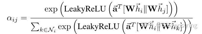 第四步:注意力加权后的结点embedding特征 第四步:注意力加权后的结点embedding特征 经过注意力加权后的结点特征embedding的代码如下: attention = F.dropout(attention, self.dropout, training=self.training) h_prime = torch.matmul(attention, Wh)这里得出的也是所有结点经过注意力加权的embedding特征,h_prime是一个 N\times F' 的矩阵,这里的attention矩阵还经过一个dropout处理。 多头注意力我们先看整个GAT神经网络的代码,代码在model.py文件中 class GAT(nn.Module): def __init__(self, nfeat, nhid, nclass, dropout, alpha, nheads): """Dense version of GAT.""" super(GAT, self).__init__() self.dropout = dropout self.attentions = [GraphAttentionLayer(nfeat, nhid, dropout=dropout, alpha=alpha, concat=True) for _ in range(nheads)] for i, attention in enumerate(self.attentions): self.add_module('attention_{}'.format(i), attention) self.out_att = GraphAttentionLayer(nhid * nheads, nclass, dropout=dropout, alpha=alpha, concat=False) def forward(self, x, adj): x = F.dropout(x, self.dropout, training=self.training) x = torch.cat([att(x, adj) for att in self.attentions], dim=1) x = F.dropout(x, self.dropout, training=self.training) x = F.elu(self.out_att(x, adj)) return F.log_softmax(x, dim=1)原论文里对多头注意力的描述用下图来表示: 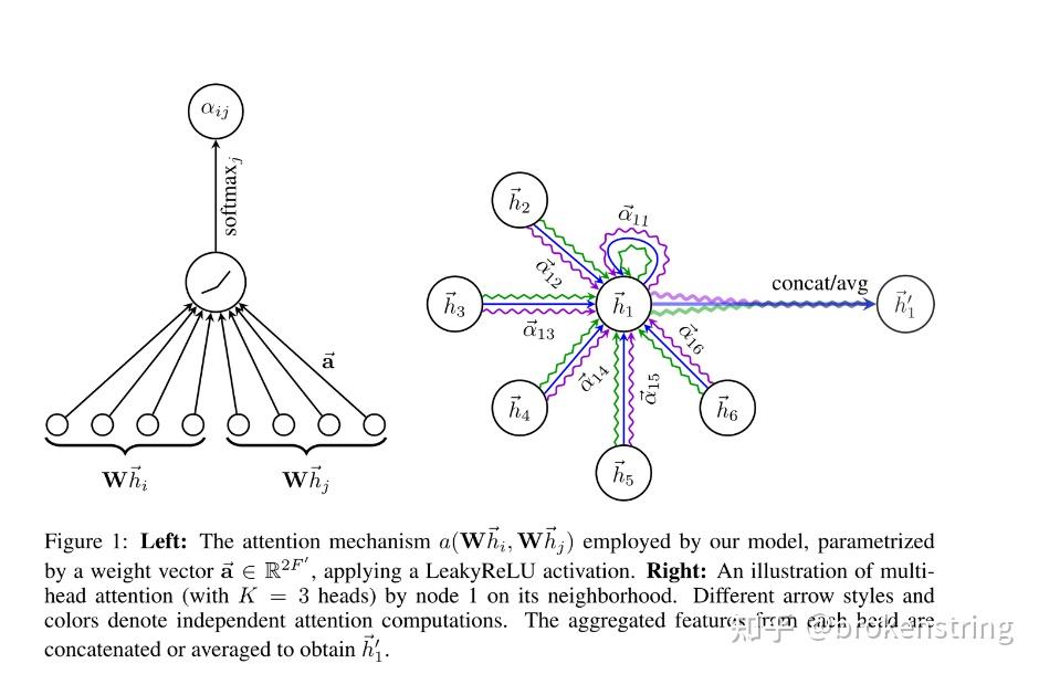 多头注意力会计算出多个 h' ,最后把这些 h' 进行均值化或者拼接一起就行。 再看源码: x = torch.cat([att(x, adj) for att in self.attentions], dim=1)首先把多头注意力的结果拼接在一起,源码中多头数为8,embedding的维度也为8,所以x是个 N\times 64 的矩阵 x = F.elu(self.out_att(x, adj))接着我们再把多头注意力拼接的结果再过一层GAT层(套着elu激活),即代码中的out_att类。out_att是由一层的GAT层定义而来的,具体定义代码为 self.out_att = GraphAttentionLayer(nhid * nheads, nclass, dropout=dropout, alpha=alpha, concat=False)这层GAT的输入维度为 64 = 8*8 维,8维的特征embedding和8头的注意力 ,输出为7维(7分类)。最后代码还经过一个log_softmax变换,方便使用似然损失函数。(注:上述讲解中忽略了一些drop_out层) 训练与预测def train(epoch): t = time.time() model.train() optimizer.zero_grad() output = model(features, adj) loss_train = F.nll_loss(output[idx_train], labels[idx_train]) acc_train = accuracy(output[idx_train], labels[idx_train]) loss_train.backward() optimizer.step() if not args.fastmode: # Evaluate validation set performance separately, # deactivates dropout during validation run. model.eval() output = model(features, adj) loss_val = F.nll_loss(output[idx_val], labels[idx_val]) acc_val = accuracy(output[idx_val], labels[idx_val]) print('Epoch: {:04d}'.format(epoch+1), 'loss_train: {:.4f}'.format(loss_train.data.item()), 'acc_train: {:.4f}'.format(acc_train.data.item()), 'loss_val: {:.4f}'.format(loss_val.data.item()), 'acc_val: {:.4f}'.format(acc_val.data.item()), 'time: {:.4f}s'.format(time.time() - t)) return loss_val.data.item() def compute_test(): model.eval() output = model(features, adj) loss_test = F.nll_loss(output[idx_test], labels[idx_test]) acc_test = accuracy(output[idx_test], labels[idx_test]) print("Test set results:", "loss= {:.4f}".format(loss_test.data.item()), "accuracy= {:.4f}".format(acc_test.data.item())) # Train model t_total = time.time() loss_values = [] bad_counter = 0 best = args.epochs + 1 best_epoch = 0 for epoch in range(args.epochs): loss_values.append(train(epoch)) torch.save(model.state_dict(), '{}.pkl'.format(epoch)) if loss_values[-1] < best: best = loss_values[-1] best_epoch = epoch bad_counter = 0 else: bad_counter += 1 if bad_counter == args.patience: break files = glob.glob('*.pkl') for file in files: epoch_nb = int(file.split('.')[0]) if epoch_nb < best_epoch: os.remove(file)这部分代码就没啥好说的了,和一般模型的训练与预测的流程差不多。代码在train.py中。 |
【本文地址】
今日新闻 |
点击排行 |
|
推荐新闻 |
图片新闻 |
|
专题文章 |