圆周运动、一般曲线运动、阿基米德螺旋线 |
您所在的位置:网站首页 › 等距螺旋线方程的推导过程 › 圆周运动、一般曲线运动、阿基米德螺旋线 |
圆周运动、一般曲线运动、阿基米德螺旋线
|
恒长旋转向量的导数
一个恒长旋转向量求导后得到的向量的方向与原向量相比,逆时针旋转了 9 0 ∘ 90^\circ 90∘ ,而求导后得到的向量的长度与旋转角速度有关。 证明例如 a ⃗ = ( c o s θ , s i n θ ) \vec{a}=(cos \ \theta, \quad sin \ \theta) a =(cos θ,sin θ) 1、对 θ \theta θ 求导 d a ⃗ d θ = ( − s i n θ , c o s θ ) = [ c o s ( θ + π 2 ) , s i n ( θ + π 2 ) ] \frac{d\vec{a}}{d\theta}=(-sin\ \theta, \quad cos \ \theta)=[cos(\theta+\frac{\pi}{2}), \quad sin(\theta+\frac{\pi}{2})] dθda =(−sin θ,cos θ)=[cos(θ+2π),sin(θ+2π)] 结论: d a ⃗ d θ \frac{d\vec{a}}{d\theta} dθda 与 a ⃗ \vec{a} a 相比,在方向上逆时针旋转了 90°,长度不变 2、对 t 求导 θ \theta θ 是关于 t t t 的函数, θ = w ⋅ t 或 θ = w ( t ) ⋅ t \theta=w \cdot t \quad 或 \quad \theta=w(t)\cdot t θ=w⋅t或θ=w(t)⋅t前者角速度恒定,后者角速度是关于时间的函数。 d a ⃗ d t = d a ⃗ d θ ⋅ d θ d t = [ d θ d t ⋅ c o s ( θ + π 2 ) , d θ d t ⋅ s i n ( θ + π 2 ) ] \frac{d\vec{a}}{dt}=\frac{d\vec{a}}{d\theta} \cdot \frac{d\theta}{dt}=[\frac{d\theta}{dt} \cdot cos(\theta+\frac{\pi}{2}), \quad \frac{d\theta}{dt} \cdot sin(\theta+\frac{\pi}{2})] dtda =dθda ⋅dtdθ=[dtdθ⋅cos(θ+2π),dtdθ⋅sin(θ+2π)] 结论: 所以, d a ⃗ d t \frac{d\vec{a}}{dt} dtda 与 a ⃗ \vec{a} a 相比,在方向上逆时针旋转了 90° ,在长度上变为原来的 w w w 倍,如果 a ⃗ \vec{a} a 作变速圆周运动, d a ⃗ d t \frac{d\vec{a}}{dt} dtda 的长度将会随时间变化。 圆周运动中角速度和线速度的关系一个质点以原点为圆心作圆周运动,设它的位移由
r
1
⃗
\vec{r_1}
r1
变成
r
2
⃗
\vec{r_2}
r2
,如下图所示 这只是大小关系,考虑方向,使用叉乘, v ⃗ = w ⃗ × r ⃗ \vec{v} = \vec{w} \times \vec{r} v =w ×r 阿基米德螺旋线 阿基米德螺旋线方程阿基米德螺旋线的极坐标方程为: r = a θ ( a > 0 ) r=a\theta \quad (a>0) r=aθ(a>0) 这表示极径与 θ \theta θ 是线性关系,成正比。 它的参数方程为: { x = r ⋅ c o s θ = a θ ⋅ c o s θ y = r ⋅ s i n θ = a θ ⋅ s i n θ \begin{cases} x=r \cdot cos \ \theta=a\theta \cdot cos \ \theta \\ y=r \cdot sin \ \theta=a\theta \cdot sin \ \theta \end{cases} {x=r⋅cos θ=aθ⋅cos θy=r⋅sin θ=aθ⋅sin θ 试图消去参数 x 2 + y 2 = ( a θ ) 2 ⋅ ( s i n 2 θ + c o s 2 θ ) = ( a θ ) 2 其 中 , θ = a r c t a n ( y x ) x^2+y^2=(a\theta)^2 \cdot (sin^2 \theta + cos^2 \theta)=(a\theta)^2 \quad 其中,\theta=arctan(\frac{y}{x}) x2+y2=(aθ)2⋅(sin2θ+cos2θ)=(aθ)2其中,θ=arctan(xy) 这个方程无法化为显函数的形式,所以,最好用极坐标方程或参数方程来表示。我们以 θ \theta θ 为参数,用 matlab 画出它的图像。 syms theta a=1; r=a*theta; x=r*cos(theta); y=r*sin(theta); fplot(x,y,[0,50],'LineWidth',1.5); grid on axis square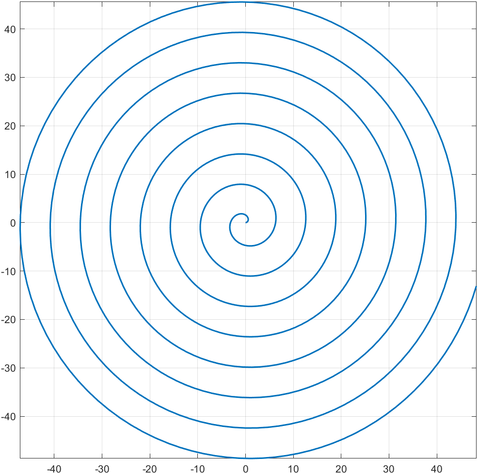 螺旋线的时间导数
设 r ⃗ \vec{r} r 为螺旋线的位移, d r ⃗ d t = d r ⃗ d θ ⋅ d θ d t \frac{d\vec{r}}{dt}=\frac{d\vec{r}}{d\theta} \cdot \frac{d\theta}{dt} dtdr =dθdr ⋅dtdθ . 可见, r ⃗ \vec{r} r 对时间求导只是对 θ \theta θ 求导后乘上一个系数 d θ d t \frac{d\theta}{dt} dtdθ 而已,所以我们研究对 θ \theta θ 的导数,而不是对 t t t 的导数。 对螺旋线的参数方程求导 syms a theta x=a*theta*cos(theta); y=a*theta*sin(theta); dx=diff(x,theta) dy=diff(y,theta)结果如下 dx = a*cos(theta) - a*theta*sin(theta) dy = a*sin(theta) + a*theta*cos(theta) >>这可以看成是两个向量的合成,分别为 ( a ⋅ c o s θ , a ⋅ s i n θ ) (a\cdot cos\ \theta,\quad a \cdot sin\ \theta) (a⋅cos θ,a⋅sin θ) 和 ( − a θ ⋅ s i n θ , a θ ⋅ c o s θ ) = [ a θ ⋅ c o s ( θ + π 2 ) , a θ ⋅ s i n ( θ + π 2 ) ] (-a\theta \cdot sin\ \theta,\quad a\theta \cdot cos \ \theta)= [a\theta \cdot cos(\theta+ \frac{\pi}{2}), \quad a\theta \cdot sin(\theta+\frac{\pi}{2})] (−aθ⋅sin θ,aθ⋅cos θ)=[aθ⋅cos(θ+2π),aθ⋅sin(θ+2π)] 分别令 { e t ⃗ = [ a θ ⋅ c o s ( θ + π 2 ) , a θ ⋅ s i n ( θ + π 2 ) ] e n ⃗ = ( a ⋅ c o s θ , a ⋅ s i n θ ) \begin{cases} \vec{e_t}=[a\theta \cdot cos(\theta+ \frac{\pi}{2}), \quad a\theta \cdot sin(\theta+\frac{\pi}{2})] \\ \vec{e_n}=(a\cdot cos\ \theta,\quad a \cdot sin\ \theta) \\ \end{cases} {et =[aθ⋅cos(θ+2π),aθ⋅sin(θ+2π)]en =(a⋅cos θ,a⋅sin θ) { v t ⃗ = d θ d t ⋅ e t ⃗ = w ⋅ e t ⃗ v n ⃗ = d θ d t ⋅ e n ⃗ = w ⋅ e n ⃗ \begin{cases} \vec{v_t}=\frac{d\theta}{dt} \cdot \vec{e_t}=w\cdot \vec{e_t} \\ \vec{v_n}=\frac{d\theta}{dt} \cdot \vec{e_n} =w\cdot \vec{e_n}\\ \end{cases} {vt =dtdθ⋅et =w⋅et vn =dtdθ⋅en =w⋅en 其中, v n ⃗ \vec{v_n} vn 的方向沿着半径向外,是法向速度, v t ⃗ \vec{v_t} vt 沿着切线,与 v n ⃗ \vec{v_n} vn 垂直,总是指向逆时针方向,是切向速度。 可以看出 w w w 恒定时,切向速度随着 θ \theta θ 的增大而增大,法向速度恒定,此时质点一方面绕着原点作圆周运动,线速度越来越大;另一方面,又以恒定的速度远离原点。 切向速度的规律这个切向速度与原来的螺旋线方程比起来有什么规律呢? 螺旋线参数方程 { x = r ⋅ c o s θ = a θ ⋅ c o s θ y = r ⋅ s i n θ = a θ ⋅ s i n θ \begin{cases} x=r \cdot cos \ \theta=a\theta \cdot cos \ \theta \\ y=r \cdot sin \ \theta=a\theta \cdot sin \ \theta \end{cases} {x=r⋅cos θ=aθ⋅cos θy=r⋅sin θ=aθ⋅sin θ 切向速度 v t ⃗ = [ a θ ⋅ c o s ( θ + π 2 ) , a θ ⋅ s i n ( θ + π 2 ) ] \vec{v_t}=[a\theta \cdot cos(\theta+ \frac{\pi}{2}), \quad a\theta \cdot sin(\theta+\frac{\pi}{2})] vt =[aθ⋅cos(θ+2π),aθ⋅sin(θ+2π)] 可以发现,切向速度与螺旋线方程比起来就是逆时针旋转了 π 2 \frac{\pi}{2} 2π 而已。 使用 matlab 画出切向速度的图像 clc; clear; close all; syms theta a=1; x=a*theta*cos(theta+pi/2); y=a*theta*sin(theta+pi/2); fplot(x,y,[0,pi*2*5],'LineWidth',1.5,'Color','b');%画出切向速度,蓝色 grid on axis square hold on x=a*theta*cos(theta); y=a*theta*sin(theta); fplot(x,y,[0,pi*2*5],'LineWidth',1.5,'Color','r');%画出阿基米德螺旋线,红色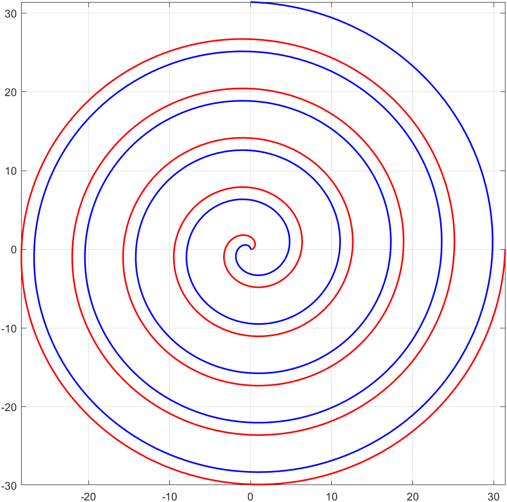
切向速度可以使用 v ⃗ = w ⃗ × r ⃗ \vec{v} = \vec{w} \times \vec{r} v =w ×r 的公式。(合速度不行) 1、使用方程组得到 v t v_t vt( v t v_t vt 的标量,即它的大小) { e t ⃗ = [ a θ ⋅ c o s ( θ + π 2 ) , a θ ⋅ s i n ( θ + π 2 ) ] e n ⃗ = ( a ⋅ c o s θ , a ⋅ s i n θ ) \begin{cases} \vec{e_t}=[a\theta \cdot cos(\theta+ \frac{\pi}{2}), \quad a\theta \cdot sin(\theta+\frac{\pi}{2})] \\ \vec{e_n}=(a\cdot cos\ \theta,\quad a \cdot sin\ \theta) \\ \end{cases} {et =[aθ⋅cos(θ+2π),aθ⋅sin(θ+2π)]en =(a⋅cos θ,a⋅sin θ) { v t ⃗ = d θ d t ⋅ e t ⃗ = w ⋅ e t ⃗ v n ⃗ = d θ d t ⋅ e n ⃗ = w ⋅ e n ⃗ \begin{cases} \vec{v_t}=\frac{d\theta}{dt} \cdot \vec{e_t}=w\cdot \vec{e_t} \\ \vec{v_n}=\frac{d\theta}{dt} \cdot \vec{e_n} =w\cdot \vec{e_n}\\ \end{cases} {vt =dtdθ⋅et =w⋅et vn =dtdθ⋅en =w⋅en 则标量方程为: { v t = w a θ = w 2 a t v n = w a \begin{cases} v_t=wa\theta =w^2at\\ v_n=wa \\ \end{cases} {vt=waθ=w2atvn=wa 2、使用 v ⃗ = w ⃗ × r ⃗ \vec{v} = \vec{w} \times \vec{r} v =w ×r 得到 v t v_t vt v t = w r = w ⋅ a θ = w a ⋅ w t = w 2 a t v_t=wr=w\cdot a\theta=wa\cdot wt=w^2at vt=wr=w⋅aθ=wa⋅wt=w2at 这两种方式得到的 v t v_t vt 一样,可见,对于任意的曲线运动,它的切向速度总是适用 v ⃗ = w ⃗ × r ⃗ \vec{v} = \vec{w} \times \vec{r} v =w ×r ,但是它的合速度不能盲目地使用这个公式。 题外话——蚊香线两条互差 180° 得阿基米德螺旋线就是蚊香得形状 clc; clear; close all; syms theta a=1; x=a*theta*cos(theta+pi); y=a*theta*sin(theta+pi); fplot(x,y,[0,pi*2*5],'LineWidth',1.5,'Color','b'); grid on axis square hold on x=a*theta*cos(theta); y=a*theta*sin(theta); fplot(x,y,[0,pi*2*5],'LineWidth',1.5,'Color','r');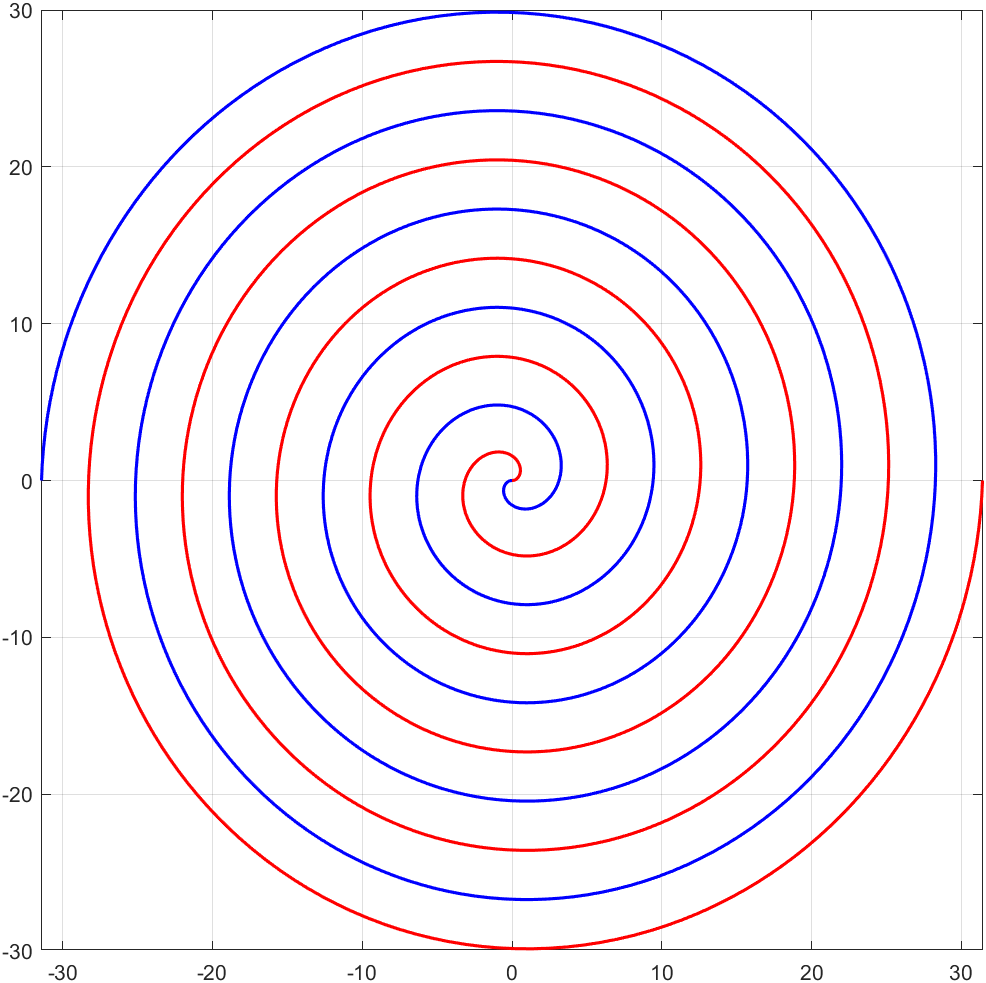
在一个平面上切割两条阿基米德螺旋线,然后横着切两刀,剩下的部分丢掉,把要的部分扒开就是两盘蚊香了。 |
 d
r
⃗
d\vec{r}
dr
是位移的变化量,
d
θ
d\theta
dθ 是弧度增量。
d
r
⃗
=
r
2
⃗
−
r
1
⃗
∣
r
1
⃗
∣
=
∣
r
2
⃗
∣
=
r
d\vec{r}=\vec{r_2}-\vec{r_1} \\ \quad \\ |\vec{r_1}|=|\vec{r_2}|=r\\
dr
=r2
−r1
∣r1
∣=∣r2
∣=r 当
d
θ
d\theta
dθ 很小时,
∣
d
r
⃗
∣
≈
弧
长
|d\vec{r}| \approx 弧长
∣dr
∣≈弧长 根据
弧
度
=
弧
长
半
径
弧度=\frac{弧长}{半径}
弧度=半径弧长 ,可得
d
θ
=
∣
d
r
⃗
∣
r
d\theta=\frac{|d\vec{r}|}{r}
dθ=r∣dr
∣,使用标量表示:
d
r
=
d
θ
⋅
r
dr=d\theta \cdot r
dr=dθ⋅r ,方程两边同时除以 dt ,得:
d
r
d
t
=
r
⋅
d
θ
d
t
\frac{dr}{dt}=r \cdot \frac{d\theta}{dt}
dtdr=r⋅dtdθ,则得到:
v
=
w
⋅
r
v=w\cdot r
v=w⋅r
d
r
⃗
d\vec{r}
dr
是位移的变化量,
d
θ
d\theta
dθ 是弧度增量。
d
r
⃗
=
r
2
⃗
−
r
1
⃗
∣
r
1
⃗
∣
=
∣
r
2
⃗
∣
=
r
d\vec{r}=\vec{r_2}-\vec{r_1} \\ \quad \\ |\vec{r_1}|=|\vec{r_2}|=r\\
dr
=r2
−r1
∣r1
∣=∣r2
∣=r 当
d
θ
d\theta
dθ 很小时,
∣
d
r
⃗
∣
≈
弧
长
|d\vec{r}| \approx 弧长
∣dr
∣≈弧长 根据
弧
度
=
弧
长
半
径
弧度=\frac{弧长}{半径}
弧度=半径弧长 ,可得
d
θ
=
∣
d
r
⃗
∣
r
d\theta=\frac{|d\vec{r}|}{r}
dθ=r∣dr
∣,使用标量表示:
d
r
=
d
θ
⋅
r
dr=d\theta \cdot r
dr=dθ⋅r ,方程两边同时除以 dt ,得:
d
r
d
t
=
r
⋅
d
θ
d
t
\frac{dr}{dt}=r \cdot \frac{d\theta}{dt}
dtdr=r⋅dtdθ,则得到:
v
=
w
⋅
r
v=w\cdot r
v=w⋅r【本文地址】
今日新闻 |
点击排行 |
|
推荐新闻 |
图片新闻 |
|
专题文章 |