Pytorch机器学习(十) |
您所在的位置:网站首页 › 无悔华夏怎么会盟失败 › Pytorch机器学习(十) |
Pytorch机器学习(十)
|
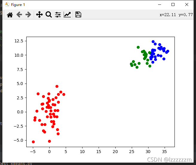
Pytorch机器学习(十)—— YOLO中k-means聚类方法生成锚框anchor 目录 Pytorch机器学习(十)—— YOLO中k-means聚类方法生成锚框anchor 前言 一、K-means聚类 k-means代码 k-means++算法 二、YOLO中使用k-means聚类生成anchor 读取VOC格式数据集 k-means聚类生成anchor 总结 前言前面文章说过有关锚框的一些知识,但有个坑一直没填,就是在YOLO中锚框的大小是如何确定出来的。其实在YOLOV3中就有采用k-means聚类方法计算锚框的方法,而在YOLOV5中作者在基于k-means聚类方法的结果之后,采用了遗传算法,进一步得到效果更好的锚框。 如果对锚框概念不理解的,可以看一下这篇文章 Pytorch机器学习(九)—— YOLO中对于锚框,预测框,产生候选区域及对候选区域进行标注详解 一、K-means聚类在YOLOV3中,锚框大小的计算就是采用的k-means聚类的方法形成的。 从直观的理解,我们知道所有已经标注的bbox的长宽大小,而锚框则是对于预测这些bbox的潜在候选框,所以锚框的长宽形状应该越接近真实bbox越好。而又由于YOLO网络的预测层是包含3种尺度的信息的(分别对应3种感受野),每种尺度的anchor又是三种,所以我们就需要9种尺度的anchor,也即我们需要对所有的bbox的尺寸聚类成9种类别!! 聚类方法比较常用的是使用k-means聚类方法,其算法流程如下。 从数据集中随机选取 K 个点作为初始聚类的中心,中心点为聚类效果如下
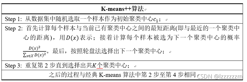
还有一种k-means++算法,是属于k-means算法的衍生吧,其主要解决的是k-means算法第一步,随机选择中心点的问题。
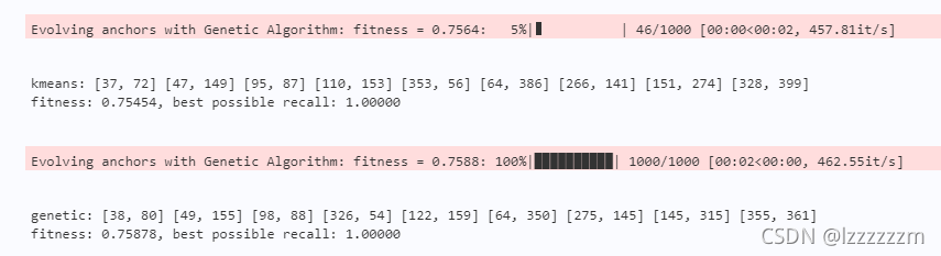
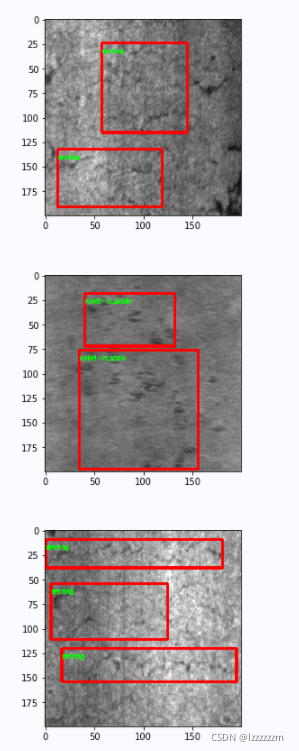
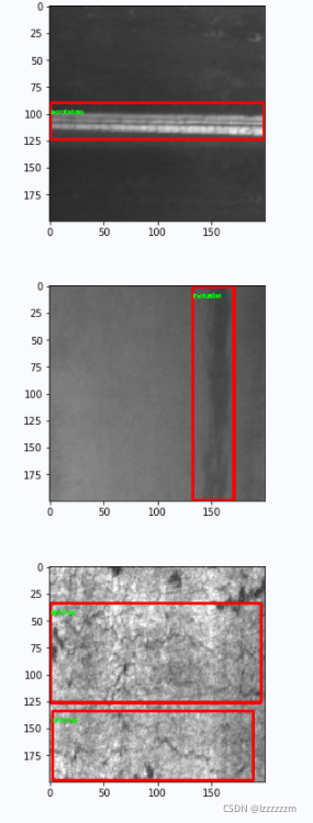
整个代码也十分简单,只需要把最先随机选取中心点用下面代码计算出来就可以。 # k_means++计算中心坐标 def calc_center(boxes): box_number = boxes.shape[0] # 随机选取第一个中心点 first_index = np.random.choice(box_number, size=1) clusters = boxes[first_index] # 计算每个样本距中心点的距离 dist_note = np.zeros(box_number) dist_note += np.inf for i in range(k): # 如果已经找够了聚类中心,则退出 if i+1 == k: break # 计算当前中心点和其他点的距离 for j in range(box_number): j_dist = single_distance(boxes[j], clusters[i]) if j_dist < dist_note[j]: dist_note[j] = j_dist # 转换为概率 dist_p = dist_note / dist_note.sum() # 使用赌轮盘法选择下一个点 next_index = np.random.choice(box_number, 1, p=dist_p) next_center = boxes[next_index] clusters = np.vstack([clusters, next_center]) return clusters但我自己在使用过程中,对于提升不大。主要因为其实bbox的尺度差异一般不会太大,所以这个中心点的选取,对于最后影响不大。 二、YOLO中使用k-means聚类生成anchor下面重点说一下如何使用这个k-means算法来生成anchor,辅助我们训练,下面的代码和上面的有一点不一样,因为我们上面的代码是基于点的(x,y),而我们聚类中,是bbox的(w,h),下面代码都以VOC格式的训练集为例,如果是coco格式的,得麻烦你自己转一下格式了。 如果不想用我下面的代码但也想用k-means聚类,请读取自己数据集时,读取bbox和图片的(w,h)以列表的形式保存,确保自己n*2或者m*2的列表. 读取VOC格式数据集我下面的代码,不仅读取了voc格式的数据集,还做了一些数据的统计,如果不想要,自己注释点就好,代码比较简单,也写了注释。 大家可以不用太纠结代码实现,记得改一下自己的图片路径即可。 from xml.dom.minidom import parse import matplotlib.pyplot as plt import cv2 as cv import os train_annotation_path = '/home/aistudio/data/train/Annotations' # 训练集annotation的路径 train_image_path = '/home/aistudio/data/train/JPEGImages' # 训练集图片的路径 # 展示图片的数目 show_num = 12 #打开xml文档 def parase_xml(xml_path): """ 输入:xml路径 返回:image_name, width, height, bboxes """ domTree = parse(xml_path) rootNode = domTree.documentElement # 得到object,sizem,图片名称属性 object_node = rootNode.getElementsByTagName("object") shape_node = rootNode.getElementsByTagName("size") image_node = rootNode.getElementsByTagName("filename") image_name = image_node[0].childNodes[0].data bboxes = [] # 解析图片的长宽 for size in shape_node: width = int(size.getElementsByTagName('width')[0].childNodes[0].data) height = int(size.getElementsByTagName('height')[0].childNodes[0].data) # 解析图片object属性 for obj in object_node: # 解析name属性,并统计类别数 class_name = obj.getElementsByTagName("name")[0].childNodes[0].data # 解析bbox属性,并统计bbox的大小 bndbox = obj.getElementsByTagName("bndbox") for bbox in bndbox: x1 = int(bbox.getElementsByTagName('xmin')[0].childNodes[0].data) y1 = int(bbox.getElementsByTagName('ymin')[0].childNodes[0].data) x2 = int(bbox.getElementsByTagName('xmax')[0].childNodes[0].data) y2 = int(bbox.getElementsByTagName('ymax')[0].childNodes[0].data) bboxes.append([class_name, x1, y1, x2, y2]) return image_name, width, height, bboxes def read_voc(train_annotation_path, train_image_path, show_num): """ train_annotation_path:训练集annotation的路径 train_image_path:训练集图片的路径 show_num:展示图片的大小 """ # 用于统计图片的长宽 total_width, total_height = 0, 0 # 用于统计图片bbox长宽 bbox_total_width, bbox_total_height, bbox_num = 0, 0, 0 min_bbox_size = 40000 max_bbox_size = 0 # 用于统计聚类所用的图片长宽,bbox长宽 img_wh = [] bbox_wh = [] # 用于统计标签 total_size = [] class_static = {'crazing': 0, 'inclusion': 0, 'patches': 0, 'pitted_surface': 0, 'rolled-in_scale': 0, 'scratches': 0} num_index = 0 for root, dirs, files in os.walk(train_annotation_path): for file in files: num_index += 1 xml_path = os.path.join(root, file) image_name, width, height, bboxes = parase_xml(xml_path) image_path = os.path.join(train_image_path, image_name) img_wh.append([width, height]) total_width += width total_height += height # 如果需要展示,则读取图片 if num_index < show_num: image_path = os.path.join(train_image_path, image_name) image = cv.imread(image_path) # 统计有关bbox的信息 wh = [] for bbox in bboxes: class_name = bbox[0] class_static[class_name] += 1 x1, y1, x2, y2 = bbox[1], bbox[2], bbox[3], bbox[4] bbox_width = x2 - x1 bbox_height = y2 - y1 bbox_size = bbox_width*bbox_height # 统计bbox的最大最小尺寸 if min_bbox_size > bbox_size: min_bbox_size = bbox_size if max_bbox_size < bbox_size: max_bbox_size = bbox_size total_size.append(bbox_size) # 统计bbox平均尺寸 bbox_total_width += bbox_width bbox_total_height += bbox_height # 用于聚类使用 wh.append([bbox_width / width, bbox_height / height]) # 相对坐标 bbox_num += 1 # 如果需要展示,绘制方框 if num_index < show_num: cv.rectangle(image, (x1, y1), (x2, y2), color=(255, 0, 0), thickness=2) cv.putText(image, class_name, (x1, y1+10), cv.FONT_HERSHEY_SIMPLEX, fontScale=0.2, color=(0, 255, 0), thickness=1) bbox_wh.append(wh) # 如果需要展示 if num_index < show_num: plt.figure() plt.imshow(image) plt.show() # 去除2个检查文件 # num_index -= 2 print("total train num is: {}".format(num_index)) print("avg total_width is {}, avg total_height is {}".format((total_width / num_index), (total_height / num_index))) print("avg bbox width is {}, avg bbox height is {} ".format((bbox_total_width / bbox_num), (bbox_total_height / bbox_num))) print("min bbox size is {}, max bbox size is {}".format(min_bbox_size, max_bbox_size)) print("class_static show below:", class_static) return img_wh, bbox_wh img_wh, bbox_wh = read_voc(train_annotation_path, train_image_path, show_num) k-means聚类生成anchor我这里的k-means代码集合了k-means++的实现,也集合了 太阳花的小绿豆这位博主提出用IOU作为评价指标来计算k-means而不是用欧拉距离的方法可以测试发现,使用IOU确实效果要比使用欧拉距离做为评价指标要好) import numpy as np # 这里IOU的概念更像是只是考虑anchor的长宽 def wh_iou(wh1, wh2): # Returns the nxm IoU matrix. wh1 is nx2, wh2 is mx2 wh1 = wh1[:, None] # [N,1,2] wh2 = wh2[None] # [1,M,2] inter = np.minimum(wh1, wh2).prod(2) # [N,M] return inter / (wh1.prod(2) + wh2.prod(2) - inter) # iou = inter / (area1 + area2 - inter) # 计算单独一个点和一个中心的距离 def single_distance(center, point): center_x, center_y = center[0]/2 , center[1]/2 point_x, point_y = point[0]/2, point[1]/2 return np.sqrt((center_x - point_x)**2 + (center_y - point_y)**2) # 计算中心点和其他点直接的距离 def calc_distance(boxes, clusters): """ :param obs: 所有的观测点 :param clusters: 中心点 :return:每个点对应中心点的距离 """ distances = [] for box in boxes: # center_x, center_y = x/2, y/2 distance = [] for center in clusters: # center_xc, cneter_yc = xc/2, yc/2 distance.append(single_distance(box, center)) distances.append(distance) return distances # k_means++计算中心坐标 def calc_center(boxes, k): box_number = boxes.shape[0] # 随机选取第一个中心点 first_index = np.random.choice(box_number, size=1) clusters = boxes[first_index] # 计算每个样本距中心点的距离 dist_note = np.zeros(box_number) dist_note += np.inf for i in range(k): # 如果已经找够了聚类中心,则退出 if i+1 == k: break # 计算当前中心点和其他点的距离 for j in range(box_number): j_dist = single_distance(boxes[j], clusters[i]) if j_dist < dist_note[j]: dist_note[j] = j_dist # 转换为概率 dist_p = dist_note / dist_note.sum() # 使用赌轮盘法选择下一个点 next_index = np.random.choice(box_number, 1, p=dist_p) next_center = boxes[next_index] clusters = np.vstack([clusters, next_center]) return clusters # k-means聚类,且评价指标采用IOU def k_means(boxes, k, dist=np.median, use_iou=True, use_pp=False): """ yolo k-means methods Args: boxes: 需要聚类的bboxes,bboxes为n*2包含w,h k: 簇数(聚成几类) dist: 更新簇坐标的方法(默认使用中位数,比均值效果略好) use_iou:是否使用IOU做为计算 use_pp:是否是同k-means++算法 """ box_number = boxes.shape[0] last_nearest = np.zeros((box_number,)) # 在所有的bboxes中随机挑选k个作为簇的中心 if not use_pp: clusters = boxes[np.random.choice(box_number, k, replace=False)] # k_means++计算初始值 else: clusters = calc_center(boxes, k) # print(clusters) while True: # 计算每个bboxes离每个簇的距离 1-IOU(bboxes, anchors) if use_iou: distances = 1 - wh_iou(boxes, clusters) else: distances = calc_distance(boxes, clusters) # 计算每个bboxes距离最近的簇中心 current_nearest = np.argmin(distances, axis=1) # 每个簇中元素不在发生变化说明以及聚类完毕 if (last_nearest == current_nearest).all(): break # clusters won't change for cluster in range(k): # 根据每个簇中的bboxes重新计算簇中心 clusters[cluster] = dist(boxes[current_nearest == cluster], axis=0) last_nearest = current_nearest return clusters使用我下面的auot_anchor代码注意!!(这里代码也是借鉴的太阳花的小绿豆博主的,他把里面的torch函数改为np函数后,使得代码移植性变强了!) 传入的参数中img_wh和bbox_wh即读取voc数据集中图片的长宽和bbox的长宽,为n*2和m*2的列表 !! 这里我还加入了YOLOV5中的遗传算法,具体细节就不展开了。 from tqdm import tqdm import random # 计算聚类和遗传算法出来的anchor和真实bbox之间的重合程度 def anchor_fitness(k: np.ndarray, wh: np.ndarray, thr: float): # mutation fitness """ 输入:k:聚类完后的结果,且排列为升序 wh:包含bbox中w,h的集合,且转换为绝对坐标 thr:bbox中和k聚类的框重合阈值 """ r = wh[:, None] / k[None] x = np.minimum(r, 1. / r).min(2) # ratio metric best = x.max(1) f = (best * (best > thr).astype(np.float32)).mean() # fitness bpr = (best > thr).astype(np.float32).mean() # best possible recall return f, bpr def auto_anchor(img_size, n, thr, gen, img_wh, bbox_wh): """ 输入:img_size:图片缩放的大小 n:聚类数 thr:fitness的阈值 gen:遗传算法迭代次数 img_wh:图片的长宽集合 bbox_wh:bbox的长框集合 """ # 最大边缩放到img_size img_wh = np.array(img_wh, dtype=np.float32) shapes = (img_size * img_wh / img_wh).max(1, keepdims=True) wh0 = np.concatenate([l * s for s, l in zip(shapes, bbox_wh)]) # wh i = (wh0 < 3.0).any(1).sum() if i: print(f'WARNING: Extremely small objects found. {i} of {len(wh0)} labels are < 3 pixels in size.') wh = wh0[(wh0 >= 2.0).any(1)] # 只保留wh都大于等于2个像素的box # k_means 聚类计算anchor k = k_means(wh, n, use_iou=True, use_pp=False) k = k[np.argsort(k.prod(1))] # sort small to large f, bpr = anchor_fitness(k, wh, thr) print("kmeans: " + " ".join([f"[{int(i[0])}, {int(i[1])}]" for i in k])) print(f"fitness: {f:.5f}, best possible recall: {bpr:.5f}") # YOLOV5改进遗传算法 npr = np.random f, sh, mp, s = anchor_fitness(k, wh, thr)[0], k.shape, 0.9, 0.1 # fitness, generations, mutation prob, sigma pbar = tqdm(range(gen), desc=f'Evolving anchors with Genetic Algorithm:') # progress bar for _ in pbar: v = np.ones(sh) while (v == 1).all(): # mutate until a change occurs (prevent duplicates) v = ((npr.random(sh) < mp) * random.random() * npr.randn(*sh) * s + 1).clip(0.3, 3.0) kg = (k.copy() * v).clip(min=2.0) fg, bpr = anchor_fitness(kg, wh, thr) if fg > f: f, k = fg, kg.copy() pbar.desc = f'Evolving anchors with Genetic Algorithm: fitness = {f:.4f}' # 按面积排序 k = k[np.argsort(k.prod(1))] # sort small to large print("genetic: " + " ".join([f"[{int(i[0])}, {int(i[1])}]" for i in k])) print(f"fitness: {f:.5f}, best possible recall: {bpr:.5f}") auto_anchor(img_size=416, n=9, thr=0.25, gen=1000, img_wh=img_wh, bbox_wh=bbox_wh)如果有兴趣代码细节的,可以看里面的注释,如果还有不懂的,可以私信我交流。 最后计算出来的结果如下,可以看到计算出来的anchor的是长方型的,这是因为我的bbox中长方型的anchor居多,符合我的预期。我们只需要把下面的anchor,替换掉默认的anchor即可!
最后说明一下,用聚类算法算出来的anchor并不一定比初始值即coco上的anchor要好,原因是目标检测大部分基于迁移学习,backbone网络的训练参数是基于coco上的anchor学习的,所以其实大部分情况用这个聚类效果并没有直接使用coco上的好!!,而且聚类效果跟数据集的数量有很大关系,一两千张图片,聚类出来效果可能不会很好 总结整个算法思路其实不难,但代码有一些冗余和长,主要也是结合自己在学习和使用过程中,发现很多博主没有说明白如何使用这些代码。 |
【本文地址】
今日新闻 |
点击排行 |
|
推荐新闻 |
图片新闻 |
|
专题文章 |