随机变量 |
您所在的位置:网站首页 › 战地5没有中文怎么办 › 随机变量 |
随机变量
统计学系列条目概率論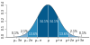 概率
概率公理
決定論
非決定論
随机性
概率空間
概率测度
样本空间
随机试验
伯努利試驗
事件
互補事件
互斥
基本事件(英语:Elementary_event)
结果
单元素
随机变量
期望值
條件概率
概率分布
離散型均勻分佈
伯努利分布
二項式分布
幾何分佈
负二项分布
超几何分布
泊松分布
连续型均匀分布
正态分布
对数正态分布
多元正态分布
指数分布
Gamma分布
Beta分布
帕累托分布
联合分布
边缘分布
随机过程
伯努利过程
隨機漫步
维纳过程
馬可夫過程
伊藤過程
統計獨立性
條件獨立
全概率公式
大数定律
贝叶斯定理
布尔不等式
文氏图
樹形圖
查论编
概率
概率公理
決定論
非決定論
随机性
概率空間
概率测度
样本空间
随机试验
伯努利試驗
事件
互補事件
互斥
基本事件(英语:Elementary_event)
结果
单元素
随机变量
期望值
條件概率
概率分布
離散型均勻分佈
伯努利分布
二項式分布
幾何分佈
负二项分布
超几何分布
泊松分布
连续型均匀分布
正态分布
对数正态分布
多元正态分布
指数分布
Gamma分布
Beta分布
帕累托分布
联合分布
边缘分布
随机过程
伯努利过程
隨機漫步
维纳过程
馬可夫過程
伊藤過程
統計獨立性
條件獨立
全概率公式
大数定律
贝叶斯定理
布尔不等式
文氏图
樹形圖
查论编
給定樣本空间 ( S , F ) {\displaystyle (S,\mathbb {F} )} ,如果其上的實值函數 X : S → R {\displaystyle X:S\to \mathbb {R} } 是 F {\displaystyle \mathbb {F} } (實值)可測函數,则稱 X {\displaystyle X} 為(實值)随机变量。初等概率論中通常不涉及到可測性的概念,而直接把任何 X : S → R {\displaystyle X:S\to \mathbb {R} } 的函數稱為随机变量。 如果 X {\displaystyle X} 指定给概率空间 S {\displaystyle S} 中每一个事件 e {\displaystyle e} 有一个实数 X ( e ) {\displaystyle X(e)} ,同时针对每一个实数 r {\displaystyle r} 都有一个事件集合 A r {\displaystyle A_{r}} 与其相对应,其中 A r = {\displaystyle A_{r}=} { e : X ( e ) {\displaystyle e:X(e)} ≤ r {\displaystyle r} },那么 X {\displaystyle X} 被称作随机变量。随机变量一般用大写拉丁字母或小写希腊字母(比如 X , Y , Z , ξ , η {\displaystyle X,Y,Z,\xi ,\eta } )来表示,从上面的定义注意到,随机变量实质上是函数。称其为变量是指可作为因变量。  实数坐标轴上的随机变量示意图 实数坐标轴上的随机变量示意图
例如,随机掷两个骰子,整个事件空间可以由36个元素组成: S = { ( i , j ) | i = 1 , … , 6 , ; j = 1 , … , 6 } {\displaystyle S=\lbrace (i,j)|i=1,\ldots ,6,;j=1,\ldots ,6\rbrace }这里可以构成多个随机变量,比如随机变量 X {\displaystyle X} (获得的两个骰子的点数和)或者随机变量 Y {\displaystyle Y} (获得的两个骰子的点数差),随机变量 X {\displaystyle X} 可以有11个整数值,而随机变量 Y {\displaystyle Y} 只有6个。 X ( i , j ) := i + j , x = 2 , 3 , … , 12 {\displaystyle X(i,j):=i+j,x=2,3,\ldots ,12} Y ( i , j ) :=∣ i − j ∣ , y = 0 , 1 , 2 , 3 , 4 , 5 {\displaystyle Y(i,j):=\mid i-j\mid ,y=0,1,2,3,4,5}又比如,在一次扔硬币事件中,如果把获得的背面的次数作为随机变量 X {\displaystyle X} ,则 X {\displaystyle X} 可以取两个值,分别是0和1。 如果随机变量 X {\displaystyle X} 的取值是有限的或者是可数无穷尽的值 X = { x 1 , x 2 , x 3 , … , } {\displaystyle X=\lbrace x_{1},x_{2},x_{3},\ldots ,\rbrace }则称 X {\displaystyle X} 为离散随机变量。 如果 X {\displaystyle X} 由全部实数或者由一部分区间组成, X = { x | a ≤ x ≤ b } {\displaystyle X=\lbrace x|a\leq x\leq b\rbrace } , − ∞ {\displaystyle \Omega } (见概率)。随机变量 X {\displaystyle X} 是定义于 Ω {\displaystyle \Omega } 上的函数,即对每一基本事件 ω ∈ Ω {\displaystyle \omega \in \Omega } ,有一数值 X ( ω ) {\displaystyle X(\omega )} 与之对应。以掷一颗骰子的随机试验为例,它的所有可能结果,共6个,分别记作 ω 1 {\displaystyle \omega _{1}} , ω 2 {\displaystyle \omega _{2}} , ω 3 {\displaystyle \omega _{3}} , ω 4 {\displaystyle \omega _{4}} , ω 5 {\displaystyle \omega _{5}} , ω 6 {\displaystyle \omega _{6}} ,这时, Ω = { ω 1 , ω 2 , ω 3 , ω 4 , ω 5 , ω 6 } {\displaystyle \Omega =\{\omega _{1},\omega _{2},\omega _{3},\omega _{4},\omega _{5},\omega _{6}\}} ,而出现的点数这个随机变量 X {\displaystyle X} ,就是 Ω {\displaystyle \Omega } 上的函数 X ( ω k ) = k {\displaystyle X(\omega k)=k} , k = 1 , 2 , … , 6 {\displaystyle k=1,2,\ldots ,6} 。又如设 Ω = { ω 1 , ω 2 , … , ω n } {\displaystyle \Omega =\{\omega _{1},\omega _{2},\ldots ,\omega _{n}\}} 是要进行抽查的 n {\displaystyle n} 个人的全体,那么随意抽查其中一人的身高和体重,就构成两个随机变量 X {\displaystyle X} 和 Y {\displaystyle Y} ,它们分别是 Ω {\displaystyle \Omega } 上的函数: X ( ω k ) = {\displaystyle X(\omega k)=} “ ω k {\displaystyle \omega k} 的身高”, Y ( ω k ) = {\displaystyle Y(\omega k)=} “ ω k {\displaystyle \omega k} 的体重”, k = 1 , 2 , … , n {\displaystyle k=1,2,\ldots ,n} 。一般说来,一个随机变量所取的值可以是离散的(如掷一颗骰子的点数只取1到6的整数,电话台收到的呼叫次数只取非负整数),也可以充满一个数值区间,或整个实数轴(如液体中悬浮的微粒沿某一方向的位移)。 研究方法[编辑]在研究随机变量的性质时,确定和计算它取某个数值或落入某个数值区间内的概率是特别重要的。因此,随机变量取某个数值或落入某个数值区间这样的基本事件的集合,应当属于所考虑的事件域。根据这样的直观想法,利用概率论公理化的语言,取实数值的随机变量的数学定义可确切地表述如下:概率空间 ( Ω , F , p ) {\displaystyle (\Omega ,F,p)} 上的随机变量 X {\displaystyle X} 是定义于 Ω {\displaystyle \Omega } 上的实值可测函数,即对任意 ω ∈ Ω {\displaystyle \omega \in \Omega } , X ( ω ) {\displaystyle X(\omega )} 为实数,且对任意实数 x {\displaystyle x} ,使 X ( ω ) ≤ x {\displaystyle X(\omega )\leq x} 的一切 ω {\displaystyle \omega } 组成的 Ω {\displaystyle \Omega } 的子集 { ω : X ( ω ) ≤ x } {\displaystyle \{\omega :X(\omega )\leq x\}} 是事件,也即是 F {\displaystyle F} 中的元素。事件 { ω : X ( ω ) ≤ x } {\displaystyle \{\omega :X(\omega )\leq x\}} 常简记作 { X ≤ x } {\displaystyle \{X\leq x\}} ,并称函数 F ( x ) = p ( X ≤ x ) {\displaystyle F(x)=p(X\leq x)} , − ∞ , F , p ) {\displaystyle (\Omega ,F,p)} 上的两个随机变量,如果除去一个零概率事件外, X ( ω ) {\displaystyle X(\omega )} 与 Y ( ω ) {\displaystyle Y(\omega )} 相同,则称 X = Y {\displaystyle X=Y} 以概率1成立,也记作 p ( X = Y ) = 1 {\displaystyle p(X=Y)=1} 或 X = Y {\displaystyle X=Y} ,α.s.(α.s.意即几乎必然)。 有些随机现象需要同时用多个随机变量来描述。例如对地面目标射击,弹着点的位置需要两个坐标才能确定,因此研究它要同时考虑两个随机变量,一般称同一概率空间 ( Ω , F , p ) {\displaystyle (\Omega ,F,p)} 上的 n {\displaystyle n} 个随机变量构成的 n {\displaystyle n} 维向量 X = ( x 1 , x 2 , … , x n ) {\displaystyle X=(x_{1},x_{2},\ldots ,x_{n})} 为 n {\displaystyle n} 维随机向量。随机变量可以看作一维随机向量。称 n {\displaystyle n} 元 x 1 , x 2 , … , x n {\displaystyle x_{1},x_{2},\ldots ,x_{n}} 的函数为 X {\displaystyle X} 的(联合)分布函数。又如果 ( x 1 , x 2 ) {\displaystyle (x_{1},x_{2})} 为二维随机向量,则称 x 1 + i x 2 ( i 2 = − 1 ) {\displaystyle x_{1}+ix_{2}(i^{2}=-1)} 为复随机变量。 随机变量的独立性 独立性是概率论所独有的一个重要概念。设 x 1 , x 2 , … , x n {\displaystyle x_{1},x_{2},\ldots ,x_{n}} 是 n {\displaystyle n} 个随机变量,如果对任何 n {\displaystyle n} 个实数 x 1 , x 2 , … , x n {\displaystyle x_{1},x_{2},\ldots ,x_{n}} 都有 即它们的联合分布函数 F ( x 1 , x 2 , … , x n ) {\displaystyle F(x_{1},x_{2},\ldots ,x_{n})} 等于它们各自的分布函数 F 1 ( x 1 ) , F 2 ( x 2 ) , … , F n ( x n ) {\displaystyle F1(x_{1}),F2(x_{2}),\ldots ,Fn(x_{n})} 的乘积。则称 x 1 , x 2 , … , x n {\displaystyle x_{1},x_{2},\ldots ,x_{n}} 是独立的。这一定义可以直接推广到每一 x k {\displaystyle xk} ( k = 1 , 2 , … , n {\displaystyle k=1,2,\ldots ,n} )是随机向量的情形。独立性的直观意义是: x 1 , x 2 , … , x n {\displaystyle x_{1},x_{2},\ldots ,x_{n}} 中的任何一个取值的概率规律,并不随其中的其他随机变量取什么值而改变。在实际问题中通常用它来表征多个独立操作的随机试验结果或多种有独立来源的随机因素的概率特性,因此它对于概率统计的应用是十分重要的。 从随机变量(或向量) x 1 , x 2 , … , x n {\displaystyle x_{1},x_{2},\ldots ,x_{n}} 的独立性还可以推出:设 B k {\displaystyle Bk} 是 x k {\displaystyle xk} 取值的空间中的任意波莱尔集, k = 1 , 2 , … , n {\displaystyle k=1,2,\ldots ,n} 。设 x 1 , x 2 , … , x n {\displaystyle x_{1},x_{2},\ldots ,x_{n}} 是独立的,则它们中的任意个都是独立的。但逆之即使其中任何 n − 1 {\displaystyle n-1} 个是独立的,也不保证 x 1 , x 2 , … , x n {\displaystyle x_{1},x_{2},\ldots ,x_{n}} 是独立的。又如果 f j ( x ) , i = 1 , 2 , … , n {\displaystyle fj(x),i=1,2,\ldots ,n} ,是 n {\displaystyle n} 个连续函数或初等函数(或更一般的波莱尔可测函数),则从 x 1 , x 2 , … , x n {\displaystyle x_{1},x_{2},\ldots ,x_{n}} 的独立性可推出 f 1 ( x 1 ) , f 2 ( x 2 ) , … , f n ( x n ) {\displaystyle f1(x_{1}),f2(x_{2}),\ldots ,fn(x_{n})} 也独立。如果随机变量(随机向量)序列 x 1 , x 2 , … , x n , … {\displaystyle x_{1},x_{2},\ldots ,x_{n},\ldots } 中任何有限个都独立,则称之为独立随机变量(随机向量)序列。 关于随机变量的矩、特征函数、母函数及半不变量,分别见数学期望、方差、動差及概率分布。 随机变量的函数[编辑]一个新的随机变量能被博雷尔 (Borel) 可测函数定义 g : R → R {\displaystyle g\colon \mathbb {R} \rightarrow \mathbb {R} } 来产生一个随机变量 X {\displaystyle X} 。 Y {\displaystyle Y} 的累积分布函数是: F Y ( y ) = P ( g ( X ) ≤ y ) . {\displaystyle F_{Y}(y)=\operatorname {P} (g(X)\leq y).}如果博雷尔函数可逆: F Y ( y ) = P ( g ( X ) ≤ y ) = { P ( X ≤ g − 1 ( y ) ) = F X ( g − 1 ( y ) ) , if g − 1 increasing , P ( X ≥ g − 1 ( y ) ) = 1 − F X ( g − 1 ( y ) ) , if g − 1 decreasing . {\displaystyle F_{Y}(y)=\operatorname {P} (g(X)\leq y)={\begin{cases}\operatorname {P} (X\leq g^{-1}(y))=F_{X}(g^{-1}(y)),&{\text{if }}g^{-1}{\text{ increasing}},\\\\\operatorname {P} (X\geq g^{-1}(y))=1-F_{X}(g^{-1}(y)),&{\text{if }}g^{-1}{\text{ decreasing}}.\end{cases}}}得到它的概率密度函数: f Y ( y ) = f X ( g − 1 ( y ) ) | d g − 1 ( y ) d y | . {\displaystyle f_{Y}(y)=f_{X}(g^{-1}(y))\left|{\frac {dg^{-1}(y)}{dy}}\right|.} 例子[编辑]定义 X {\displaystyle X} 为实数,在连续性随机变量里,让 Y = X 2 {\displaystyle Y=X^{2}} F Y ( y ) = P ( X 2 ≤ y ) . {\displaystyle F_{Y}(y)=\operatorname {P} (X^{2}\leq y).}如果 y 0 {\displaystyle y\geq 0} P ( X 2 ≤ y ) = P ( | X | ≤ y ) = P ( − y ≤ X ≤ y ) , {\displaystyle \operatorname {P} (X^{2}\leq y)=\operatorname {P} (|X|\leq {\sqrt {y}})=\operatorname {P} (-{\sqrt {y}}\leq X\leq {\sqrt {y}}),}可以得到: F Y ( y ) = F X ( y ) − F X ( − y ) if y ≥ 0. {\displaystyle F_{Y}(y)=F_{X}({\sqrt {y}})-F_{X}(-{\sqrt {y}})\qquad {\hbox{if}}\quad y\geq 0.} 參考文獻[编辑] Fristedt, Bert; Gray, Lawrence. A modern approach to probability theory. Boston: Birkhäuser. 1996 [2017-03-01]. ISBN 3-7643-3807-5. (原始内容存档于2021-04-28). Kallenberg, Olav. Random Measures 4th. Berlin: Akademie Verlag. 1986 [2017-03-01]. ISBN 0-12-394960-2. MR 0854102. (原始内容存档于2021-05-01). 引文格式1维护:MR格式 (link) Kallenberg, Olav. Foundations of Modern Probability 2nd. Berlin: Springer Verlag. 2001 [2017-03-01]. ISBN 0-387-95313-2. (原始内容存档于2021-04-02). Papoulis, Athanasios. Probability, Random Variables, and Stochastic Processes 9th. Tokyo: McGraw–Hill. 1965 [2017-03-01]. ISBN 0-07-119981-0. (原始内容存档于2017-06-26). 外部链接[编辑] Hazewinkel, Michiel (编), Random variable, 数学百科全书, Springer, 2001, ISBN 978-1-55608-010-4 Zukerman, Moshe, Introduction to Queueing Theory and Stochastic Teletraffic Models (PDF), 2014 [2017-03-01], (原始内容 (PDF)存档于2016-08-11) Zukerman, Moshe, Basic Probability Topics (PDF), 2014 [2017-03-01], (原始内容 (PDF)存档于2021-04-02) 參見[编辑] 概率论 隨機分佈 隨機性 隨機向量 隨機函數 生成函數 算法信息论 随机变量的收敛 查论编统计学描述统计学连续概率集中趋势平均数(平方 · 算術 · 幾何 · 調和 · 算术-几何 · 几何-调和 · 希羅/平均数不等式) · 中位數 · 眾數离散程度全距 · 变异系数 · 百分位數 · 四分位距 · 四分位数 · 標準差 · 方差 · 平均差 · 標準分數 · 切比雪夫不等式 · 基尼系数分布形态(英语:Shape of the distribution)中心极限定理 · 矩(偏態 · 峰態)离散概率次數(英语:Count data) · 列聯表(英语:Contingency table) 推論統計學和假說檢定推論統計學置信区间 · 區間估計(英语:Interval estimation) · 显著性差异 · 元分析 · 贝叶斯推断实验设计总体 · 抽樣 · 重抽样(刀切法 · 自助法 · 交叉驗證) · 重复(英语:Replication (statistics)) · 阻碍 · 靈敏度和特異度 · 區集(英语:Blocking (statistics)) · 缺失数据样本量(英语:Sample size)標準誤 · 零假设 · 备择假设 · 第一类错误与第二类错误 · 统计功效 · 效应值常规估计贝叶斯推断 · 區間估計(英语:Interval estimation) · 最大似然估计 · 最小距離估計(英语:Minimum distance estimation) · 矩估计 · 最大间距假设检验Z檢驗 · 学生t检验 · F檢定 · 卡方检验 · Wald檢定(英语:Wald test) · 曼-惠特尼檢定(英语:Mann–Whitney U test) · 秩和检验生存分析生存函数 · 乘積極限估計量 · 對數秩和檢定 · 失效率 · 危險比例模式相關及迴歸分析相关性干擾因素 · 皮尔逊積矩相關係數 · 等級相關(英语:Rank correlation) (斯皮尔曼等级相关系数 · 肯德等級相關係數(英语:Kendall tau rank correlation coefficient)) · 自由度 · 误差和残差線性回歸線性模型(英语:Linear model) · 一般线性模型 · 廣義線性模型 · 简单线性回归(英语:Simple linear regression) · 普通最小二乘法 · 贝叶斯回归(英语:Bayesian linear regression) · 方差分析 · 协方差分析(英语:Analysis of covariance)非线性回归非参数回归模型(英语:Nonparametric regression) · 半参数回归模型(英语:Semiparametric regression) · 邏輯迴歸统计图形饼图 · 条形图 · 双标图 · 箱形圖 · 管制圖 · 森林圖(英语:Forest plot) · 直方图 · 分位圖 · 趋势图 · 散点图 · 莖葉圖 · 雷达图(英语:Radar chart) · 示意地圖其他回應過程效度 · 統計誤用 推論統計學和假說檢定推論統計學置信区间 · 區間估計(英语:Interval estimation) · 显著性差异 · 元分析 · 贝叶斯推断实验设计总体 · 抽樣 · 重抽样(刀切法 · 自助法 · 交叉驗證) · 重复(英语:Replication (statistics)) · 阻碍 · 靈敏度和特異度 · 區集(英语:Blocking (statistics)) · 缺失数据样本量(英语:Sample size)標準誤 · 零假设 · 备择假设 · 第一类错误与第二类错误 · 统计功效 · 效应值常规估计贝叶斯推断 · 區間估計(英语:Interval estimation) · 最大似然估计 · 最小距離估計(英语:Minimum distance estimation) · 矩估计 · 最大间距假设检验Z檢驗 · 学生t检验 · F檢定 · 卡方检验 · Wald檢定(英语:Wald test) · 曼-惠特尼檢定(英语:Mann–Whitney U test) · 秩和检验生存分析生存函数 · 乘積極限估計量 · 對數秩和檢定 · 失效率 · 危險比例模式相關及迴歸分析相关性干擾因素 · 皮尔逊積矩相關係數 · 等級相關(英语:Rank correlation) (斯皮尔曼等级相关系数 · 肯德等級相關係數(英语:Kendall tau rank correlation coefficient)) · 自由度 · 误差和残差線性回歸線性模型(英语:Linear model) · 一般线性模型 · 廣義線性模型 · 简单线性回归(英语:Simple linear regression) · 普通最小二乘法 · 贝叶斯回归(英语:Bayesian linear regression) · 方差分析 · 协方差分析(英语:Analysis of covariance)非线性回归非参数回归模型(英语:Nonparametric regression) · 半参数回归模型(英语:Semiparametric regression) · 邏輯迴歸统计图形饼图 · 条形图 · 双标图 · 箱形圖 · 管制圖 · 森林圖(英语:Forest plot) · 直方图 · 分位圖 · 趋势图 · 散点图 · 莖葉圖 · 雷达图(英语:Radar chart) · 示意地圖其他回應過程效度 · 統計誤用
|
 ,如果其上的實值函數
X
:
S
→
R
{\displaystyle X:S\to \mathbb {R} }
,如果其上的實值函數
X
:
S
→
R
{\displaystyle X:S\to \mathbb {R} }
 是
F
{\displaystyle \mathbb {F} }
是
F
{\displaystyle \mathbb {F} }
 (實值)可測函數,则稱
X
{\displaystyle X}
(實值)可測函數,则稱
X
{\displaystyle X}
 為(實值)随机变量。初等概率論中通常不涉及到可測性的概念,而直接把任何
X
:
S
→
R
{\displaystyle X:S\to \mathbb {R} }
為(實值)随机变量。初等概率論中通常不涉及到可測性的概念,而直接把任何
X
:
S
→
R
{\displaystyle X:S\to \mathbb {R} }
 中每一个事件
e
{\displaystyle e}
中每一个事件
e
{\displaystyle e}
 有一个实数
X
(
e
)
{\displaystyle X(e)}
有一个实数
X
(
e
)
{\displaystyle X(e)}
 ,同时针对每一个实数
r
{\displaystyle r}
,同时针对每一个实数
r
{\displaystyle r}
 都有一个事件集合
A
r
{\displaystyle A_{r}}
都有一个事件集合
A
r
{\displaystyle A_{r}}
 与其相对应,其中
A
r
=
{\displaystyle A_{r}=}
与其相对应,其中
A
r
=
{\displaystyle A_{r}=}
 {
e
:
X
(
e
)
{\displaystyle e:X(e)}
{
e
:
X
(
e
)
{\displaystyle e:X(e)}
 ≤
r
{\displaystyle r}
≤
r
{\displaystyle r}
 )来表示,从上面的定义注意到,随机变量实质上是函数。称其为变量是指可作为因变量。

 (获得的两个骰子的点数差),随机变量
X
{\displaystyle X}
(获得的两个骰子的点数差),随机变量
X
{\displaystyle X}
 Y
(
i
,
j
)
:=∣
i
−
j
∣
,
y
=
0
,
1
,
2
,
3
,
4
,
5
{\displaystyle Y(i,j):=\mid i-j\mid ,y=0,1,2,3,4,5}
Y
(
i
,
j
)
:=∣
i
−
j
∣
,
y
=
0
,
1
,
2
,
3
,
4
,
5
{\displaystyle Y(i,j):=\mid i-j\mid ,y=0,1,2,3,4,5}


 ,
−
∞
{\displaystyle \Omega }
,
−
∞
{\displaystyle \Omega }
 (见概率)。随机变量
X
{\displaystyle X}
(见概率)。随机变量
X
{\displaystyle X}
 ,有一数值
X
(
ω
)
{\displaystyle X(\omega )}
,有一数值
X
(
ω
)
{\displaystyle X(\omega )}
 与之对应。以掷一颗骰子的随机试验为例,它的所有可能结果,共6个,分别记作
ω
1
{\displaystyle \omega _{1}}
与之对应。以掷一颗骰子的随机试验为例,它的所有可能结果,共6个,分别记作
ω
1
{\displaystyle \omega _{1}}
 ,
ω
2
{\displaystyle \omega _{2}}
,
ω
2
{\displaystyle \omega _{2}}
 ,
ω
3
{\displaystyle \omega _{3}}
,
ω
3
{\displaystyle \omega _{3}}
 ,
ω
4
{\displaystyle \omega _{4}}
,
ω
4
{\displaystyle \omega _{4}}
 ,
ω
5
{\displaystyle \omega _{5}}
,
ω
5
{\displaystyle \omega _{5}}
 ,
ω
6
{\displaystyle \omega _{6}}
,
ω
6
{\displaystyle \omega _{6}}
 ,这时,
Ω
=
{
ω
1
,
ω
2
,
ω
3
,
ω
4
,
ω
5
,
ω
6
}
{\displaystyle \Omega =\{\omega _{1},\omega _{2},\omega _{3},\omega _{4},\omega _{5},\omega _{6}\}}
,这时,
Ω
=
{
ω
1
,
ω
2
,
ω
3
,
ω
4
,
ω
5
,
ω
6
}
{\displaystyle \Omega =\{\omega _{1},\omega _{2},\omega _{3},\omega _{4},\omega _{5},\omega _{6}\}}
 ,而出现的点数这个随机变量
X
{\displaystyle X}
,而出现的点数这个随机变量
X
{\displaystyle X}
 ,
k
=
1
,
2
,
…
,
6
{\displaystyle k=1,2,\ldots ,6}
,
k
=
1
,
2
,
…
,
6
{\displaystyle k=1,2,\ldots ,6}
 。又如设
Ω
=
{
ω
1
,
ω
2
,
…
,
ω
n
}
{\displaystyle \Omega =\{\omega _{1},\omega _{2},\ldots ,\omega _{n}\}}
。又如设
Ω
=
{
ω
1
,
ω
2
,
…
,
ω
n
}
{\displaystyle \Omega =\{\omega _{1},\omega _{2},\ldots ,\omega _{n}\}}
 是要进行抽查的
n
{\displaystyle n}
是要进行抽查的
n
{\displaystyle n}
 个人的全体,那么随意抽查其中一人的身高和体重,就构成两个随机变量
X
{\displaystyle X}
个人的全体,那么随意抽查其中一人的身高和体重,就构成两个随机变量
X
{\displaystyle X}
 “
ω
k
{\displaystyle \omega k}
“
ω
k
{\displaystyle \omega k}
 的身高”,
Y
(
ω
k
)
=
{\displaystyle Y(\omega k)=}
的身高”,
Y
(
ω
k
)
=
{\displaystyle Y(\omega k)=}
 “
ω
k
{\displaystyle \omega k}
“
ω
k
{\displaystyle \omega k}
 。一般说来,一个随机变量所取的值可以是离散的(如掷一颗骰子的点数只取1到6的整数,电话台收到的呼叫次数只取非负整数),也可以充满一个数值区间,或整个实数轴(如液体中悬浮的微粒沿某一方向的位移)。
研究方法[编辑]
。一般说来,一个随机变量所取的值可以是离散的(如掷一颗骰子的点数只取1到6的整数,电话台收到的呼叫次数只取非负整数),也可以充满一个数值区间,或整个实数轴(如液体中悬浮的微粒沿某一方向的位移)。
研究方法[编辑]
 上的随机变量
X
{\displaystyle X}
上的随机变量
X
{\displaystyle X}
 ,使
X
(
ω
)
≤
x
{\displaystyle X(\omega )\leq x}
,使
X
(
ω
)
≤
x
{\displaystyle X(\omega )\leq x}
 的一切
ω
{\displaystyle \omega }
的一切
ω
{\displaystyle \omega }
 组成的
Ω
{\displaystyle \Omega }
组成的
Ω
{\displaystyle \Omega }
 是事件,也即是
F
{\displaystyle F}
是事件,也即是
F
{\displaystyle F}
 中的元素。事件
{
ω
:
X
(
ω
)
≤
x
}
{\displaystyle \{\omega :X(\omega )\leq x\}}
中的元素。事件
{
ω
:
X
(
ω
)
≤
x
}
{\displaystyle \{\omega :X(\omega )\leq x\}}
 ,并称函数
F
(
x
)
=
p
(
X
≤
x
)
{\displaystyle F(x)=p(X\leq x)}
,并称函数
F
(
x
)
=
p
(
X
≤
x
)
{\displaystyle F(x)=p(X\leq x)}
 ,
−
∞
,
F
,
p
)
{\displaystyle (\Omega ,F,p)}
,
−
∞
,
F
,
p
)
{\displaystyle (\Omega ,F,p)}
 相同,则称
X
=
Y
{\displaystyle X=Y}
相同,则称
X
=
Y
{\displaystyle X=Y}
 以概率1成立,也记作
p
(
X
=
Y
)
=
1
{\displaystyle p(X=Y)=1}
以概率1成立,也记作
p
(
X
=
Y
)
=
1
{\displaystyle p(X=Y)=1}
 或
X
=
Y
{\displaystyle X=Y}
或
X
=
Y
{\displaystyle X=Y}
 为
n
{\displaystyle n}
为
n
{\displaystyle n}
 的函数为
X
{\displaystyle X}
的函数为
X
{\displaystyle X}
 为二维随机向量,则称
x
1
+
i
x
2
(
i
2
=
−
1
)
{\displaystyle x_{1}+ix_{2}(i^{2}=-1)}
为二维随机向量,则称
x
1
+
i
x
2
(
i
2
=
−
1
)
{\displaystyle x_{1}+ix_{2}(i^{2}=-1)}
 为复随机变量。
随机变量的独立性 独立性是概率论所独有的一个重要概念。设
x
1
,
x
2
,
…
,
x
n
{\displaystyle x_{1},x_{2},\ldots ,x_{n}}
为复随机变量。
随机变量的独立性 独立性是概率论所独有的一个重要概念。设
x
1
,
x
2
,
…
,
x
n
{\displaystyle x_{1},x_{2},\ldots ,x_{n}}
 等于它们各自的分布函数
F
1
(
x
1
)
,
F
2
(
x
2
)
,
…
,
F
n
(
x
n
)
{\displaystyle F1(x_{1}),F2(x_{2}),\ldots ,Fn(x_{n})}
等于它们各自的分布函数
F
1
(
x
1
)
,
F
2
(
x
2
)
,
…
,
F
n
(
x
n
)
{\displaystyle F1(x_{1}),F2(x_{2}),\ldots ,Fn(x_{n})}
 的乘积。则称
x
1
,
x
2
,
…
,
x
n
{\displaystyle x_{1},x_{2},\ldots ,x_{n}}
的乘积。则称
x
1
,
x
2
,
…
,
x
n
{\displaystyle x_{1},x_{2},\ldots ,x_{n}}
 (
k
=
1
,
2
,
…
,
n
{\displaystyle k=1,2,\ldots ,n}
(
k
=
1
,
2
,
…
,
n
{\displaystyle k=1,2,\ldots ,n}
 是
x
k
{\displaystyle xk}
是
x
k
{\displaystyle xk}
 个是独立的,也不保证
x
1
,
x
2
,
…
,
x
n
{\displaystyle x_{1},x_{2},\ldots ,x_{n}}
个是独立的,也不保证
x
1
,
x
2
,
…
,
x
n
{\displaystyle x_{1},x_{2},\ldots ,x_{n}}
 ,是
n
{\displaystyle n}
,是
n
{\displaystyle n}
 也独立。如果随机变量(随机向量)序列
x
1
,
x
2
,
…
,
x
n
,
…
{\displaystyle x_{1},x_{2},\ldots ,x_{n},\ldots }
也独立。如果随机变量(随机向量)序列
x
1
,
x
2
,
…
,
x
n
,
…
{\displaystyle x_{1},x_{2},\ldots ,x_{n},\ldots }
 中任何有限个都独立,则称之为独立随机变量(随机向量)序列。
关于随机变量的矩、特征函数、母函数及半不变量,分别见数学期望、方差、動差及概率分布。
中任何有限个都独立,则称之为独立随机变量(随机向量)序列。
关于随机变量的矩、特征函数、母函数及半不变量,分别见数学期望、方差、動差及概率分布。
 来产生一个随机变量
X
{\displaystyle X}
来产生一个随机变量
X
{\displaystyle X}


 例子[编辑]


 參考文獻[编辑]
Fristedt, Bert; Gray, Lawrence. A modern approach to probability theory. Boston: Birkhäuser. 1996 [2017-03-01]. ISBN 3-7643-3807-5. (原始内容存档于2021-04-28).
Kallenberg, Olav. Random Measures 4th. Berlin: Akademie Verlag. 1986 [2017-03-01]. ISBN 0-12-394960-2. MR 0854102. (原始内容存档于2021-05-01). 引文格式1维护:MR格式 (link)
Kallenberg, Olav. Foundations of Modern Probability 2nd. Berlin: Springer Verlag. 2001 [2017-03-01]. ISBN 0-387-95313-2. (原始内容存档于2021-04-02).
Papoulis, Athanasios. Probability, Random Variables, and Stochastic Processes 9th. Tokyo: McGraw–Hill. 1965 [2017-03-01]. ISBN 0-07-119981-0. (原始内容存档于2017-06-26).
外部链接[编辑]
Hazewinkel, Michiel (编), Random variable, 数学百科全书, Springer, 2001, ISBN 978-1-55608-010-4
Zukerman, Moshe, Introduction to Queueing Theory and Stochastic Teletraffic Models (PDF), 2014 [2017-03-01], (原始内容 (PDF)存档于2016-08-11)
Zukerman, Moshe, Basic Probability Topics (PDF), 2014 [2017-03-01], (原始内容 (PDF)存档于2021-04-02)
參見[编辑]
概率论
隨機分佈
隨機性
隨機向量
隨機函數
生成函數
算法信息论
随机变量的收敛
查论编统计学描述统计学连续概率集中趋势平均数(平方 · 算術 · 幾何 · 調和 · 算术-几何 · 几何-调和 · 希羅/平均数不等式) · 中位數 · 眾數离散程度全距 · 变异系数 · 百分位數 · 四分位距 · 四分位数 · 標準差 · 方差 · 平均差 · 標準分數 · 切比雪夫不等式 · 基尼系数分布形态(英语:Shape of the distribution)中心极限定理 · 矩(偏態 · 峰態)离散概率次數(英语:Count data) · 列聯表(英语:Contingency table)
參考文獻[编辑]
Fristedt, Bert; Gray, Lawrence. A modern approach to probability theory. Boston: Birkhäuser. 1996 [2017-03-01]. ISBN 3-7643-3807-5. (原始内容存档于2021-04-28).
Kallenberg, Olav. Random Measures 4th. Berlin: Akademie Verlag. 1986 [2017-03-01]. ISBN 0-12-394960-2. MR 0854102. (原始内容存档于2021-05-01). 引文格式1维护:MR格式 (link)
Kallenberg, Olav. Foundations of Modern Probability 2nd. Berlin: Springer Verlag. 2001 [2017-03-01]. ISBN 0-387-95313-2. (原始内容存档于2021-04-02).
Papoulis, Athanasios. Probability, Random Variables, and Stochastic Processes 9th. Tokyo: McGraw–Hill. 1965 [2017-03-01]. ISBN 0-07-119981-0. (原始内容存档于2017-06-26).
外部链接[编辑]
Hazewinkel, Michiel (编), Random variable, 数学百科全书, Springer, 2001, ISBN 978-1-55608-010-4
Zukerman, Moshe, Introduction to Queueing Theory and Stochastic Teletraffic Models (PDF), 2014 [2017-03-01], (原始内容 (PDF)存档于2016-08-11)
Zukerman, Moshe, Basic Probability Topics (PDF), 2014 [2017-03-01], (原始内容 (PDF)存档于2021-04-02)
參見[编辑]
概率论
隨機分佈
隨機性
隨機向量
隨機函數
生成函數
算法信息论
随机变量的收敛
查论编统计学描述统计学连续概率集中趋势平均数(平方 · 算術 · 幾何 · 調和 · 算术-几何 · 几何-调和 · 希羅/平均数不等式) · 中位數 · 眾數离散程度全距 · 变异系数 · 百分位數 · 四分位距 · 四分位数 · 標準差 · 方差 · 平均差 · 標準分數 · 切比雪夫不等式 · 基尼系数分布形态(英语:Shape of the distribution)中心极限定理 · 矩(偏態 · 峰態)离散概率次數(英语:Count data) · 列聯表(英语:Contingency table)【本文地址】
今日新闻 |
点击排行 |
|
推荐新闻 |
图片新闻 |
|
专题文章 |