XGBOOST从原理到实战:二分类 、多分类 |
您所在的位置:网站首页 › 二分类损失函数的代码 › XGBOOST从原理到实战:二分类 、多分类 |
XGBOOST从原理到实战:二分类 、多分类
|
注:转载请注明出处,https://blog.csdn.net/HHTNAN/ 文章目录 XGboost完整系统的原理+实战:[课程直通车](https://edu.csdn.net/course/detail/10332)1.XGBoost2. XGBoost的优点2.1 正则化2.2 并行处理2.3 灵活性2.4 缺失值处理2.5 剪枝2.6 内置交叉验证 3. XGBoost详解3.1 数据格式3.2 参数设置3.3xgboost 模型训练方法和参数 4.模型的训练、预测、保存4.1 训练模型4.3 保存与加载模型 5. XGBoost参数说明5.1 General Parameters5.2 Parameters for Tree Booster5.3 Parameter for Linear Booster5.4 Task Parameters 6. XGBoost实战特征重要性 多分类两大类接口基于XGBoost原生接口的分类基于XGBoost原生接口的回归基于Scikit-learn接口的分类基于Scikit-learn接口的回归 XGboost完整系统的原理+实战:课程直通车 ##### 数据topK ```python a = np.array([1,4,3,5,2]) K=4 #返回索引 print(a[np.argpartition(-a,K)][:3]) #返回排序后的结果 print( a[np.argsort(-a)][:3]) ```
1.XGBoost
##### 数据topK ```python a = np.array([1,4,3,5,2]) K=4 #返回索引 print(a[np.argpartition(-a,K)][:3]) #返回排序后的结果 print( a[np.argsort(-a)][:3]) ```
1.XGBoost
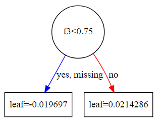
xgboost是大规模并行boosted tree的工具,它是目前最快最好的开源boosted tree工具包,比常见的工具包快10倍以上。在数据科学方面,有大量kaggle选手选用它进行数据挖掘比赛,其中包括两个以上kaggle比赛的夺冠方案。在工业界规模方面,xgboost的分布式版本有广泛的可移植性,支持在YARN, MPI, Sungrid Engine等各个平台上面运行,并且保留了单机并行版本的各种优化,使得它可以很好地解决于工业界规模的问题。 下载地址:直通车 2. XGBoost的优点 2.1 正则化XGBoost在代价函数里加入了正则项,用于控制模型的复杂度。正则项里包含了树的叶子节点个数、每个叶子节点上输出的score的L2模的平方和。从Bias-variance tradeoff角度来讲,正则项降低了模型的variance,使学习出来的模型更加简单,防止过拟合,这也是xgboost优于传统GBDT的一个特性。 2.2 并行处理XGBoost工具支持并行。Boosting不是一种串行的结构吗?怎么并行的?注意XGBoost的并行不是tree粒度的并行,XGBoost也是一次迭代完才能进行下一次迭代的(第t次迭代的代价函数里包含了前面t-1次迭代的预测值)。XGBoost的并行是在特征粒度上的。 我们知道,决策树的学习最耗时的一个步骤就是对特征的值进行排序(因为要确定最佳分割点),XGBoost在训练之前,预先对数据进行了排序,然后保存为block结构,后面的迭代中重复地使用这个结构,大大减小计算量。这个block结构也使得并行成为了可能,在进行节点的分裂时,需要计算每个特征的增益,最终选增益最大的那个特征去做分裂,那么各个特征的增益计算就可以开多线程进行。 2.3 灵活性XGBoost支持用户自定义目标函数和评估函数,只要目标函数二阶可导就行。 2.4 缺失值处理对于特征的值有缺失的样本,xgboost可以自动学习出它的分裂方向 2.5 剪枝XGBoost 先从顶到底建立所有可以建立的子树,再从底到顶反向进行剪枝。比起GBM,这样不容易陷入局部最优解。 2.6 内置交叉验证XGBoost允许在每一轮boosting迭代中使用交叉验证。因此,可以方便地获得最优boosting迭代次数。而GBM使用网格搜索,只能检测有限个值。 3. XGBoost详解 3.1 数据格式XGBoost可以加载多种数据格式的训练数据: libsvm 格式的文本数据; Numpy 的二维数组; XGBoost 的二进制的缓存文件。加载的数据存储在对象 DMatrix 中 下面一一列举: 加载libsvm格式的数据 dtrain1 = xgb.DMatrix('train.svm.txt')加载numpy的数组 data = np.random.rand(5,10) # 5 entities, each contains 10 features label = np.random.randint(2, size=5) # binary target dtrain = xgb.DMatrix( data, label=label)将scipy.sparse格式的数据转化为 DMatrix 格式 csr = scipy.sparse.csr_matrix( (dat, (row,col)) ) dtrain = xgb.DMatrix( csr )将 DMatrix 格式的数据保存成XGBoost的二进制格式,在下次加载时可以提高加载速度,使用方式如下 dtrain = xgb.DMatrix('train.svm.txt') dtrain.save_binary("train.buffer")可以用如下方式处理 DMatrix中的缺失值: dtrain = xgb.DMatrix( data, label=label, missing = -999.0)当需要给样本设置权重时,可以用如下方式 w = np.random.rand(5,1) dtrain = xgb.DMatrix( data, label=label, missing = -999.0, weight=w) 3.2 参数设置XGBoost使用key-value字典的方式存储参数: params = { 'booster': 'gbtree', 'objective': 'multi:softmax', # 多分类的问题 'num_class': 10, # 类别数,与 multisoftmax 并用 'gamma': 0.1, # 用于控制是否后剪枝的参数,越大越保守,一般0.1、0.2这样子。 'max_depth': 12, # 构建树的深度,越大越容易过拟合 'lambda': 2, # 控制模型复杂度的权重值的L2正则化项参数,参数越大,模型越不容易过拟合。 'subsample': 0.7, # 随机采样训练样本 'colsample_bytree': 0.7, # 生成树时进行的列采样 'min_child_weight': 3, 'silent': 1, # 设置成1则没有运行信息输出,最好是设置为0. 'eta': 0.007, # 如同学习率 'seed': 1000, 'nthread': 4, # cpu 线程数 } 3.3xgboost 模型训练方法和参数在训练过程中主要用到两个方法:xgboost.train()和xgboost.cv(). #xgboost.train()API xgboost.train(params,dtrain,num_boost_round=10,evals=(),obj=None,feval=None,maximize=False,early_stopping_rounds=None, evals_result=None,verbose_eval=True,learning_rates=None,xgb_model=None) params 这是一个字典,里面包含着训练中的参数关键字和对应的值,形式是params = {‘booster’:’gbtree’,’eta’:0.1}dtrain 训练的数据num_boost_round 这是指提升迭代的个数evals 这是一个列表,用于对训练过程中进行评估列表中的元素。形式是evals = [(dtrain,’train’),(dval,’val’)]或者是evals = [(dtrain,’train’)],对于第一种情况,它使得我们可以在训练过程中观察验证集的效果。obj,自定义目的函数feval,自定义评估函数maximize ,是否对评估函数进行最大化early_stopping_rounds,早期停止次数,假设为100,验证集的误差迭代到一定程度在100次内不能再继续降低,就停止迭代。这要求evals 里至少有 一个元素,如果有多个,按最后一个去执行。返回的是最后的迭代次数(不是最好的)。如果early_stopping_rounds 存在,则模型会生成三个属性,bst.best_score,bst.best_iteration,和bst.best_ntree_limit evals_result 字典,存储在watchlist 中的元素的评估结果。verbose_eval (可以输入布尔型或数值型),也要求evals 里至少有 一个元素。如果为True ,则对evals中元素的评估结果会输出在结果中;如果输入数字,假设为5,则每隔5个迭代输出一次。learning_rates 每一次提升的学习率的列表,xgb_model ,在训练之前用于加载的xgb model。参数初步定之后划分20%为验证集,准备一个watchlist 给train和validation set ,设置num_round 足够大(比如100000),以至于你能发现每一个round 的验证集预测结果,如果在某一个round后 validation set 的预测误差上升了,你就可以停止掉正在运行的程序了。 watchlist = [(dtrain,'train'),(dval,'val')] model = xgb.train(params,dtrain,num_boost_round=100000,evals = watchlist) 4.模型的训练、预测、保存 4.1 训练模型有了参数列表和数据就可以训练模型了 num_round = 10 bst = xgb.train( plst, dtrain, num_round, evallist )#####4.2模型预测 # X_test类型可以是二维List,也可以是numpy的数组 dtest = DMatrix(X_test) ans = model.predict(dtest) 4.3 保存与加载模型在训练完成之后可以将模型保存下来,也可以查看模型内部的结构 bst.save_model('test.model')加载模型 通过如下方式可以加载模型: bst = xgb.Booster({'nthread':4}) # init model bst.load_model("model.bin") # load data 4.4导出模型和特征映射(Map)你可以导出模型到txt文件并浏览模型的含义: # dump model bst.dump_model('dump.raw.txt') # dump model with feature map bst.dump_model('dump.raw.txt','featmap.txt') 5. XGBoost参数说明在运行XGboost之前,必须设置三种类型成熟:general parameters,booster parameters和task parameters: General parameters该参数参数控制在提升(boosting)过程中使用哪种booster,常用的booster有树模型(tree)和线性模型(linear model)。 Booster parameters这取决于使用哪种booster。 Task parameters控制学习的场景,例如在回归问题中会使用不同的参数控制排序。 5.1 General Parameters booster [default=gbtree]有两中模型可以选择gbtree和gblinear。gbtree使用基于树的模型进行提升计算,gblinear使用线性模型进行提升计算。缺省值为gbtree silent [default=0] 取0时表示打印出运行时信息,取1时表示以缄默方式运行,不打印运行时信息。缺省值为0 nthreadXGBoost运行时的线程数。缺省值是当前系统可以获得的最大线程数 num_pbuffer预测缓冲区大小,通常设置为训练实例的数目。缓冲用于保存最后一步提升的预测结果,无需人为设置。 num_featureBoosting过程中用到的特征维数,设置为特征个数。XGBoost会自动设置,无需人为设置。 5.2 Parameters for Tree Booster eta [default=0.3]为了防止过拟合,更新过程中用到的收缩步长。在每次提升计算之后,算法会直接获得新特征的权重。 eta通过缩减特征的权重使提升计算过程更加保守。缺省值为0.3 取值范围为:[0,1] gamma [default=0]minimum loss reduction required to make a further partition on a leaf node of the tree. the larger, the more conservative the algorithm will be. 取值范围为:[0,∞] max_depth [default=6]数的最大深度。缺省值为6 取值范围为:[1,∞] min_child_weight [default=1]子节点中最小的样本权重和。如果一个叶子节点的样本权重和小于min_child_weight则拆分过程结束。在现行回归模型中,这个参数是指建立每个模型所需要的最小样本数。该成熟越大算法越conservative 取值范围为:[0,∞] max_delta_step [default=0]我们允许每个树的权重被估计的值。如果它的值被设置为0,意味着没有约束;如果它被设置为一个正值,它能够使得更新的步骤更加保守。通常这个参数是没有必要的,但是如果在逻辑回归中类极其不平衡这时候他有可能会起到帮助作用。把它范围设置为1-10之间也许能控制更新。 取值范围为:[0,∞] subsample [default=1]用于训练模型的子样本占整个样本集合的比例。如果设置为0.5则意味着XGBoost将随机的从整个样本集合中随机的抽取出50%的子样本建立树模型,这能够防止过拟合。 取值范围为:(0,1] colsample_bytree [default=1]在建立树时对特征采样的比例。缺省值为1 取值范围为:(0,1] 5.3 Parameter for Linear Booster lambda [default=0]L2 正则的惩罚系数 alpha [default=0]L1 正则的惩罚系数 lambda_bias在偏置上的L2正则。缺省值为0(在L1上没有偏置项的正则,因为L1时偏置不重要) 5.4 Task Parameters objective [ default=reg:linear ]定义学习任务及相应的学习目标,可选的目标函数如下: “reg:linear” —— 线性回归。 “reg:logistic”—— 逻辑回归。 “binary:logistic”—— 二分类的逻辑回归问题,输出为概率。 “binary:logitraw”—— 二分类的逻辑回归问题,输出的结果为wTx。 “count:poisson”—— 计数问题的poisson回归,输出结果为poisson分布。在poisson回归中,max_delta_step的缺省值为0.7。(used to safeguard optimization) “multi:softmax” –让XGBoost采用softmax目标函数处理多分类问题,同时需要设置参数num_class(类别个数) “multi:softprob” –和softmax一样,但是输出的是ndata * nclass的向量,可以将该向量reshape成ndata行nclass列的矩阵。没行数据表示样本所属于每个类别的概率。 “rank:pairwise” –set XGBoost to do ranking task by minimizing the pairwise loss base_score [ default=0.5 ]所有实例的初始化预测分数,全局偏置; 为了足够的迭代次数,改变这个值将不会有太大的影响。 eval_metric [ default according to objective ]校验数据所需要的评价指标,不同的目标函数将会有缺省的评价指标(rmse for regression, and error for classification, mean average precision for ranking) 用户可以添加多种评价指标,对于Python用户要以list传递参数对给程序,而不是map参数list参数不会覆盖’eval_metric’ 可供的选择如下: “rmse”: root mean square error “logloss”: negative log-likelihood “error”: Binary classification error rate. It is calculated as #(wrong cases)/#(all cases). For the predictions, the evaluation will regard the instances with prediction value larger than 0.5 as positive instances, and the others as negative instances. “merror”: Multiclass classification error rate. It is calculated as #(wrongcases)#(allcases). “mlogloss”: Multiclass logloss “auc”: Area under the curve for ranking evaluation. “ndcg”:Normalized Discounted Cumulative Gain “map”:Mean average precision “ndcg@n”,”map@n”: n can be assigned as an integer to cut off the top positions in the lists for evaluation. “ndcg-“,”map-“,”ndcg@n-“,”map@n-“: In XGBoost, NDCG and MAP will evaluate the score of a list without any positive samples as 1. By adding “-” in the evaluation metric XGBoost will evaluate these score as 0 to be consistent under some conditions. training repeatively seed [ default=0 ]随机数的种子。缺省值为0 6. XGBoost实战XGBoost有两大类接口:XGBoost原生接口 和 scikit-learn接口 ,并且XGBoost能够实现 分类 和 回归 两种任务。对于分类任务,XGBOOST可以实现二分类和多分类,本文从这两个方向入手: #####二分类 """ 使用鸢尾花的数据来说明二分类的问题 """ from sklearn import datasets iris = datasets.load_iris() data = iris.data[:100] print (data.shape) #一共有100个样本数据, 维度为4维 label = iris.target[:100] print (label)(100, 4) [0 0 0 0 0 0 0 0 0 0 0 0 0 0 0 0 0 0 0 0 0 0 0 0 0 0 0 0 0 0 0 0 0 0 0 0 0 0 0 0 0 0 0 0 0 0 0 0 0 0 1 1 1 1 1 1 1 1 1 1 1 1 1 1 1 1 1 1 1 1 1 1 1 1 1 1 1 1 1 1 1 1 1 1 1 1 1 1 1 1 1 1 1 1 1 1 1 1 1 1] 上面分类为0-1二分类,接下来进行模型的预测与评估 from sklearn.cross_validation import train_test_split train_x, test_x, train_y, test_y = train_test_split(data, label, random_state=0) import xgboost as xgb dtrain=xgb.DMatrix(train_x,label=train_y) dtest=xgb.DMatrix(test_x) params={'booster':'gbtree', 'objective': 'binary:logistic', 'eval_metric': 'auc', 'max_depth':4, 'lambda':10, 'subsample':0.75, 'colsample_bytree':0.75, 'min_child_weight':2, 'eta': 0.025, 'seed':0, 'nthread':8, 'silent':1} watchlist = [(dtrain,'train')] bst=xgb.train(params,dtrain,num_boost_round=5,evals=watchlist) #输出概率 ypred=bst.predict(dtest) # 设置阈值, 输出一些评价指标,选择概率大于0.5的为1,其他为0类 y_pred = (ypred ;= 0.5)*1 from sklearn import metrics print ('AUC: %.4f' % metrics.roc_auc_score(test_y,ypred)) print ('ACC: %.4f' % metrics.accuracy_score(test_y,y_pred)) print ('Recall: %.4f' % metrics.recall_score(test_y,y_pred)) print ('F1-score: %.4f' %metrics.f1_score(test_y,y_pred)) print ('Precesion: %.4f' %metrics.precision_score(test_y,y_pred)) print(metrics.confusion_matrix(test_y,y_pred))[0] train-auc:1 [1] train-auc:1 [2] train-auc:1 [3] train-auc:1 [4] train-auc:1 AUC: 1.0000 ACC: 1.0000 Recall: 1.0000 F1-score: 1.0000 Precesion: 1.0000 [[13 0] [ 0 12]] ######所属的叶子节点 当设置pred_leaf=True的时候, 这时就会输出每个样本在所有树中的叶子节点 ypred_leaf = bst.predict(dtest, pred_leaf=True)[[1 1 1 1 1] [2 2 2 2 2] [1 1 1 1 1] … [2 2 2 2 2] [1 1 1 1 1]] 输出的维度为[样本数, 树的数量], 树的数量默认是100, 所以ypred_leaf的维度为[100*100].对于第一行数据的解释就是, 在xgboost所有的100棵树里, 预测的叶子节点都是1(相对于每颗树).那怎么看每颗树以及相应的叶子节点的分值呢?这里有两种方法, 可视化树或者直接输出模型. xgb.to_graphviz(bst, num_trees=0) #可视化第一棵树的生成情况) #直接输出模型的迭代工程 bst.dump_model("model.txt")
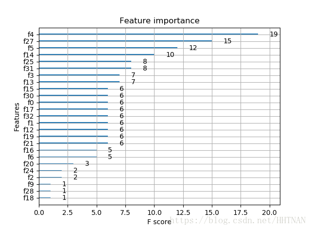
[0] train-merror:0.023438 test-merror:0.063636 [1] train-merror:0.015625 test-merror:0.045455 [2] train-merror:0.015625 test-merror:0.036364 [3] train-merror:0.007813 test-merror:0.036364 [4] train-merror:0.007813 test-merror:0.036364 [5] train-merror:0.007813 test-merror:0.018182 predicting, classification error=0.018182 #2.probabilities # do the same thing again, but output probabilities param['objective'] = 'multi:softprob' bst = xgb.train(param, xg_train, num_round, watchlist ); # Note: this convention has been changed since xgboost-unity # get prediction, this is in 1D array, need reshape to (ndata, nclass) yprob = bst.predict( xg_test ).reshape( y_test.shape[0], 6 ) #从预测的6组中选择最大的概率进行输出 ylabel = np.argmax(yprob, axis=1) # return the index of the biggest pro print ('predicting, classification error=%f' % (sum( int(ylabel[i]) != y_test[i] for i in range(len(y_test))) / float(len(y_test)) )) #最小二乘方差 mse2 = mean_squared_error(y_test,ylabel) print(mse2)[0] train-merror:0.023438 test-merror:0.063636 [1] train-merror:0.015625 test-merror:0.045455 [2] train-merror:0.015625 test-merror:0.036364 [3] train-merror:0.007813 test-merror:0.036364 [4] train-merror:0.007813 test-merror:0.036364 [5] train-merror:0.007813 test-merror:0.018182 predicting, classification error=0.018182 0.07272727272727272 from sklearn import metrics print ('ACC: %.4f' % metrics.accuracy_score(y_test,ylabel)) print(metrics.confusion_matrix(y_test,ylabel))ACC: 0.9818 [[27 0 0 0 0 0] [ 0 19 0 1 0 0] [ 0 0 21 0 0 0] [ 0 1 0 17 0 0] [ 0 0 0 0 16 0] [ 0 0 0 0 0 8]] 显示重要特征 plot_importance(bst) plt.show()####django2.0.5调用 参见链接:https://blog.csdn.net/HHTNAN/article/details/80894247 参考文献: 文献1 文献2 文献3 文献4 文献5 文献6 文献7 |
 booster[0]: 0:[f2}
# use softmax multi-class classification
param['objective'] = 'multi:softmax'
# scale weight of positive examples
param['eta'] = 0.1
param['max_depth'] = 6
param['silent'] = 1
param['nthread'] = 4
param['num_class'] = 6
watchlist = [ (xg_train,'train'), (xg_test, 'test') ]
num_round = 6
bst = xgb.train(param, xg_train, num_round, watchlist );
pred = bst.predict( xg_test );
print ('predicting, classification error=%f' % (sum( int(pred[i]) != y_test[i] for i in range(len(y_test))) / float(len(y_test)) ))
booster[0]: 0:[f2}
# use softmax multi-class classification
param['objective'] = 'multi:softmax'
# scale weight of positive examples
param['eta'] = 0.1
param['max_depth'] = 6
param['silent'] = 1
param['nthread'] = 4
param['num_class'] = 6
watchlist = [ (xg_train,'train'), (xg_test, 'test') ]
num_round = 6
bst = xgb.train(param, xg_train, num_round, watchlist );
pred = bst.predict( xg_test );
print ('predicting, classification error=%f' % (sum( int(pred[i]) != y_test[i] for i in range(len(y_test))) / float(len(y_test)) ))
【本文地址】
今日新闻 |
点击排行 |
|
推荐新闻 |
图片新闻 |
|
专题文章 |