Solve Differential Equations with ODEINT |
您所在的位置:网站首页 › solve_ivp与odeint区别 › Solve Differential Equations with ODEINT |
Solve Differential Equations with ODEINT
     Differential equations are solved in Python with the Scipy.integrate package using function odeint or solve_ivp.  Jupyter Notebook ODEINT Examples on GitHub Jupyter Notebook ODEINT Examples on GitHub
 Jupyter Notebook ODEINT Examples in Google Colab Jupyter Notebook ODEINT Examples in Google Colab
ODEINT requires three inputs: y = odeint(model, y0, t) model: Function name that returns derivative values at requested y and t values as dydt = model(y,t) y0: Initial conditions of the differential states t: Time points at which the solution should be reported. Additional internal points are often calculated to maintain accuracy of the solution but are not reported.An example of using ODEINT is with the following differential equation with parameter k=0.3, the initial condition y0=5 and the following differential equation. $$\frac{dy(t)}{dt} = -k \; y(t)$$ The Python code first imports the needed Numpy, Scipy, and Matplotlib packages. The model, initial conditions, and time points are defined as inputs to ODEINT to numerically calculate y(t). import numpy as np from scipy.integrate import odeint import matplotlib.pyplot as plt # function that returns dy/dt def model(y,t): k = 0.3 dydt = -k * y return dydt # initial condition y0 = 5 # time points t = np.linspace(0,20) # solve ODE y = odeint(model,y0,t) # plot results plt.plot(t,y) plt.xlabel('time') plt.ylabel('y(t)') plt.show() [$[Get Code]]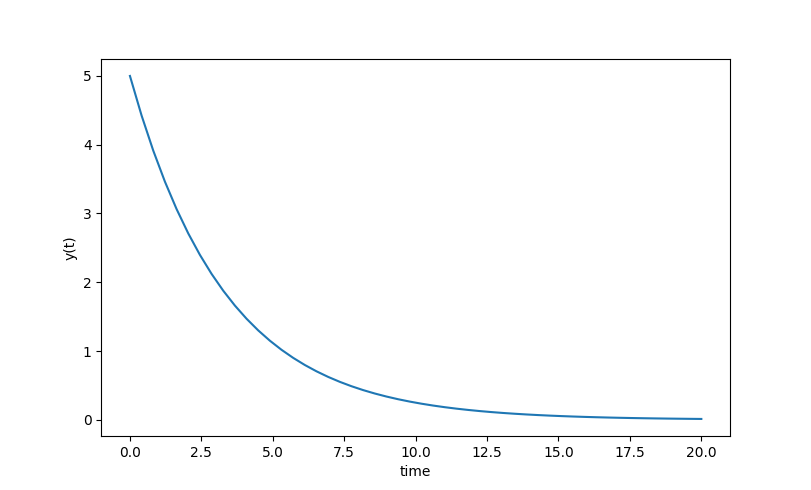
An optional fourth input is args that allows additional information to be passed into the model function. The args input is a tuple sequence of values. The argument k is now an input to the model function by including an addition argument. import numpy as np from scipy.integrate import odeint import matplotlib.pyplot as plt # function that returns dy/dt def model(y,t,k): dydt = -k * y return dydt # initial condition y0 = 5 # time points t = np.linspace(0,20) # solve ODEs k = 0.1 y1 = odeint(model,y0,t,args=(k,)) k = 0.2 y2 = odeint(model,y0,t,args=(k,)) k = 0.5 y3 = odeint(model,y0,t,args=(k,)) # plot results plt.plot(t,y1,'r-',linewidth=2,label='k=0.1') plt.plot(t,y2,'b--',linewidth=2,label='k=0.2') plt.plot(t,y3,'g:',linewidth=2,label='k=0.5') plt.xlabel('time') plt.ylabel('y(t)') plt.legend() plt.show() [$[Get Code]]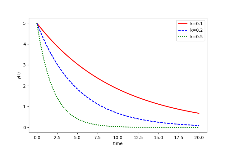 Exercises
Find a numerical solution to the following differential equations with the associated initial conditions. Expand the requested time horizon until the solution reaches a steady state. Show a plot of the states (x(t) and/or y(t)). Report the final value of each state as `t \to \infty`. Problem 1 $$\frac{dy(t)}{dt} = -y(t) + 1$$ $$y(0) = 0$$
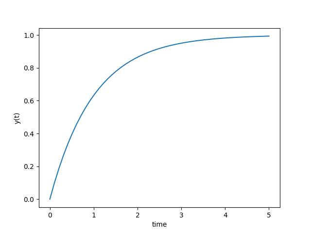 import numpy as np
from scipy.integrate import odeint
import matplotlib.pyplot as plt
# function that returns dy/dt
def model(y,t):
dydt = -y + 1.0
return dydt
# initial condition
y0 = 0
# time points
t = np.linspace(0,5)
# solve ODE
y = odeint(model,y0,t)
# plot results
plt.plot(t,y)
plt.xlabel('time')
plt.ylabel('y(t)')
plt.show()
[$[Get Code]]
import numpy as np
from scipy.integrate import odeint
import matplotlib.pyplot as plt
# function that returns dy/dt
def model(y,t):
dydt = -y + 1.0
return dydt
# initial condition
y0 = 0
# time points
t = np.linspace(0,5)
# solve ODE
y = odeint(model,y0,t)
# plot results
plt.plot(t,y)
plt.xlabel('time')
plt.ylabel('y(t)')
plt.show()
[$[Get Code]]
Problem 2 $$5 \; \frac{dy(t)}{dt} = -y(t) + u(t)$$ $$y(0) = 1$$ `u` steps from 0 to 2 at `t=10`
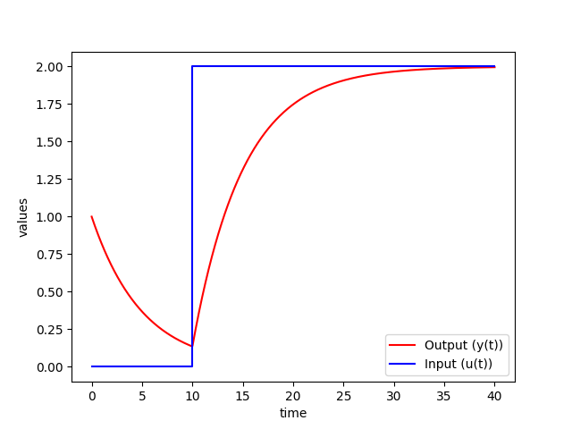 import numpy as np
from scipy.integrate import odeint
import matplotlib.pyplot as plt
# function that returns dy/dt
def model(y,t):
# u steps from 0 to 2 at t=10
if t
import numpy as np
from scipy.integrate import odeint
import matplotlib.pyplot as plt
# function that returns dy/dt
def model(y,t):
# u steps from 0 to 2 at t=10
if t |
【本文地址】
今日新闻 |
点击排行 |
|
推荐新闻 |
图片新闻 |
|
专题文章 |