系统辨识 Identification Algorithm（基础篇）

您所在的位置：网站首页 › 遗忘曲线法背知识点可以吗 › 系统辨识 Identification Algorithm（基础篇）

系统辨识 Identification Algorithm（基础篇）

2024-06-04 04:54| 来源: 网络整理| 查看: 265

基础知识

什么是系统辨识

辨识模型

噪声

矩阵运算

模型

时间序列模型 Time series model

方程误差模型 Equation error type model

输出误差模型 Output error type model

最小二乘法 Least Squares Principle

迭代最小二乘辨识 RLS identification

迭代最小二乘辨识的推导（对ARX模型）

最终结论

几个重要概念

带遗忘因子的迭代最小二乘辨识算法 FF-RLS

数据饱和

带遗忘因子的 RLS

固定记忆的 RLS

基础篇总结

基础知识什么是系统辨识

根据测得的输入输出，通过最小化误差标准函数，确定数学模型中未知的参数取值

Identification can be defined as the determination of a mathematical model from the observed input and output data by minimizing some error criterion function.

四个基本要素：

A data set 数据集

A set of candidate models 模型类

criterion function 指标函数

optimizaiton approaches 优化方法

辨识模型

在传递函数中，我们常用微分算子 s 的分式来表达输入输出之间的关系。在系统辨识中，我们根据移位算子 z 的差分方程来表达输入、输出、噪声之间的关系

$\begin{align*} &forward \ shift \ operator \ zu(t)= u(t+1)\\ &backward \ shift \ operator \ z^{-1}u(t)=u(t-1)\\\ \end{align*}$

在系统辨识算法中，为了让不同的情况，不同的算法有共通的体系结构，我们所有的算法均是基于辨识模型(identification model) 进行推演

$y(t)=H_t\theta+v(t)\quad where\ v(t)\ is\ white\ noise$

辨识模型的特点：无参变量\已知量 = 带参变量*待辨识参数 + 白噪声

噪声

随机变量：形容随机事件的数学描述

随机过程：随时间变化的随机变量，依赖于时间 t 和事件 w，当时间固定时，即随机变量

白噪声 White Noise：

$\begin{align*} &1)expectation \ is\ zero :Ev(t)=0\\ &2)variance \ Ev^{2}(t) \ is \ time \ invariant\\ &3)E(v(t)-Ev(t))(v(\tau)-Ev(\tau))=0\\ \end{align*}$

Question: which terms as follows belong to white noise if v(t) is white noise:

$\begin{align*} &A.zv(t)\\ &B.z^{-1}v(t)\\ &C.av(t)\\ &D.(a+bz^{-1})v(t)\\ \end{align*}$

根据白噪声的定义和性质可知，ABC仍然属于白噪声，而D不满足第三个条件

矩阵运算 f 列向量对 x 列向量的偏导：

$\frac{\partial f}{\partial x}= \left[ \begin{array}{cccc} \frac{\partial f_{1}}{\partial x_{1}} & \frac{\partial f_{2}}{\partial x_{1}} &... &\frac{\partial f_{m}}{\partial x_{1}}\\ \frac{\partial f_{1}}{\partial x_{2}} & \frac{\partial f_{2}}{\partial x_{2}} &... &\frac{\partial f_{m}}{\partial x_{2}}\\ ... &... &\ &...\\ \frac{\partial f_{1}}{\partial x_{n}} & \frac{\partial f_{2}}{\partial x_{n}} &... &\frac{\partial f_{m}}{\partial x_{n}}\\ \end{array} \right ]$

f 标量对 x 列向量的偏导：

$\frac{\partial f}{\partial x}=\left[ \begin{array}{cccc} \frac{\partial f}{\partial x_{1}}\\ \frac{\partial f}{\partial x_{2}}\\ ...\\ \frac{\partial f}{\partial x_{n}}\\ \end{array} \right ]$

f 列向量对 x 标量的偏导：

$\frac{\partial f}{\partial x}=\left[ \begin{array}{cccc} \frac{\partial f_{1}}{\partial x}\\ \frac{\partial f_{2}}{\partial x}\\ ...\\ \frac{\partial f_{m}}{\partial x}\\ \end{array} \right ]$

lemma 1

$\begin{align*} Given \ A \in \mathbb{R}^{n \times n},f(x)=x^{T}Ax,one\ has\\ \frac{\partial f}{\partial x}=Ax+A^{T}x \end{align*}$

lemma 2

$\begin{align*} Given \ A \in \mathbb{R}^{m \times n},f(x)=Ax,one\ has\\ \frac{\partial f}{\partial x}=A^{T} \end{align*}$

链导法则 chain rule

$\begin{align*} &Let \ x= \left[ \begin{array}{cccc} x_{1}\\x_{2}\\...\\x_{n} \end{} \right ] \ y= \left[ \begin{array}{cccc} y_{1}\\y_{2}\\...\\y_{r} \end{} \right ] \ z= \left[ \begin{array}{cccc} z_{1}\\z_{2}\\...\\z_{m} \end{} \right ]\\ &where \ z \ is \ a \ function \ of \ y,which \ is \ in\ turn\ a\ function\ of\ x.Then,\\ &\qquad \qquad \qquad \frac{\partial z}{\partial x}=\frac{\partial y}{\partial x}\frac{\partial z}{\partial y} \end{align*}$

模型

系统辨识中的模型均采用差分方程 difference function 的形式表达，其中

$\begin{align*} A(z)=1+\sum\limits_{i=1}^{n_{a}}{a_{i}z^{-i}},\quad B(z)=\sum\limits_{i=1}^{n_{b}}{b_{i}z^{-i}},\quad C(z)=\sum\limits_{i=1}^{n_{c}}{c_{i}z^{-i}},\quad D(z)=\sum\limits_{i=1}^{n_{d}}{d_{i}z^{-i}},\\ \end{align*}$

常用模型如下

时间序列模型 Time series model 自回归模型 AutoRegressive (AR) model

$\begin{align*} y(t)+a_{1}y(t-1)+a_{2}y(t-2)+...+a_{n_{a}}y(t-n_{a})&=v(t)\\ A(z)y(t)&=v(t)\\ \end{align*}$

其中，v是白噪声，na是自回归信号的阶

滑动平均模型 Moving Average (MA) model

$\begin{align*} y(t)&=v(t)+d_{1}v(t-1)+d_{2}v(t-2)+...+d_{n_{d}}v(t-n_{d})\\ y(t)&=D(z)v(t)\\ \end{align*}$

自回归滑动平均模型 AutoRegressive Moving Average (ARMA) model

$\begin{align*} y(t)+a_{1}y(t-1)+a_{2}y(t-2)+...+a_{n_{a}}y(t-n_{a})&=v(t)+d_{1}v(t-1)+d_{2}v(t-2)+...+d_{n_{d}}v(t-n_{d})\\ A(z)y(t)&=D(z)v(t)\\ \end{align*}$

确定性ARMA模型 Deterministic ARMA (DARMA) model

$\begin{align*} y(t)+a_{1}y(t-1)+a_{2}y(t-2)+...+a_{n_{a}}y(t-n_{a})&=u(t)+b_{1}u(t-1)+b_{2}u(t-2)+...+b_{n_{b}}u(t-n_{b})\\ A(z)y(t)&=B(z)u(t)\\ \end{align*}$

自回归整合滑动平均模型 AutoRegressive Integtated Moving Average (ARIMA) model

$\begin{align*} A(z)(1-z^{-1})^{d}y(t)&=D(z)v(t)\\ \end{align*}$

方程误差模型 Equation error type model

以下命名中的字母分别对应，输出信号类型、噪声类型、输入X

$\begin{align*} General:\quad &A(z)y(t)=B(z)u(t)+w(t)\\ARX: \quad &A(z)y(t)=B(z)u(t)+v(t)\\ ARMAX: \quad &A(z)y(t)=B(z)u(t)+\frac{1}{C(z)}v(t)\\ ARARMA(BJ): \quad &A(z)y(t)=B(z)u(t)+\frac{D(z)}{C(z)}v(t)\\ \end{align*}$

输出误差模型 Output error type model

以下命名中的字母分别对应，输出OE、输入类型、噪声类型

$\begin{align*} General:\quad &y(t)=\frac{B(z)}{A(z)}u(t)+w(t)\\OE: \quad &y(t)=\frac{B(z)}{A(z)}u(t)+v(t)\\ OEMA: \quad &y(t)=\frac{B(z)}{A(z)}u(t)+D(z)v(t)\\ OEARMA(BJ): \quad &y(t)=\frac{B(z)}{A(z)}u(t)+\frac{D(z)}{C(z)}v(t)\\ \end{align*}$

最小二乘法 Least Squares Principle

此章为最小二乘法的推导过程，作为系统辨识算法推理的基础，详见最小二乘估计

迭代最小二乘辨识 RLS identification

最小二乘辨识算法的核心，在于将现有模型转化为辨识模型(identification model) 用以参数辨识

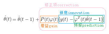
$y(t)=H_t\theta+v(t)\quad where\ v(t)\ is\ white\ noise$

迭代最小二乘辨识的推导（对ARX模型）

$\begin{align*} A(z)y(t)&=B(z)u(t)+v(t)\\ A(z)&=1+\sum_{i=1}^{n_a}{a_iz^{-i}};\quad B(z)=1+\sum_{i=1}^{n_b}{b_i}z^{-i}\\ we \ define \ \theta&=[a_1 \quad a_2 \quad ... \quad a_{n_{a}} \quad b_1 \quad b_2 \quad ... \quad b_{n_{b}}];\\ \varphi(t)&=[-y(t-1) \quad -y(t-2) \quad ... \quad -y(t-n_a) \quad u(t-1) \quad u(t-2) \quad ... \quad u(t-n_b)]; \end{}$

为了凑成辨识模型，我们定义 θ 和 φ 以便后期计算，可得相应的辨识模型

$\begin{align*} Y_t=\left[ \begin{align*} y(1)\\y(2)\\...\\y(t) \end{} \right ]\in\mathbb{R}^t,\ H_t&=\left[ \begin{align*} \varphi^T(1)\\\varphi^T(2)\\...\\\varphi^T(t) \end{} \right ]\in\mathbb{R}^{t \times n},\ V_t= \left[ \begin{align*} v(1)\\v(2)\\...\\v(t) \end{} \right ]\in\mathbb{R}^t,\\ identification\ model:\ Y_t&=H_t\theta+V_t\\ quadratic\ criterion\ function:\ J(\theta)&=V_t^TV_t\\ &=(Y_t-H_t\theta)^T(Y_t-H_t\theta) \end{}$

根据最小二乘法中得到的结论，参数 θ 的最小二乘估计为 $\hat{\theta}(t)=\hat{\theta}_{LS}(t)=(H^T_tH_t)^{-1}H^T_tY_t$

据此，将 LSE 中求逆的部分单独定义为 $P(t)=(H^T_tH_t)^{-1}$

为了保证算法的递推性，需要将 LSE 中的各变量递推关系式写出，如下

$\begin{align*} P^{-1}(t)&=H^T_tH_t=\sum_{i=1}^{t}{\varphi(i)\varphi^T(i)}=P^{-1}(t-1)+\varphi^T(t)\varphi(t)\tag{1.1}\\ Y_t&=\left[\begin{array}{ccccc} y(1)\\y(2)\\...\\y(t-1)\\y(t) \end{}\right]=\left[\begin{array}{cc} Y_{t-1}\\y(t) \end{}\right]\in\mathbb{R}^t;\\ H_t&=\left[\begin{array}{ccccc} \varphi^T(1)\\\varphi^T(2)\\...\\\varphi^T(t-1)\\\varphi^T(t) \end{}\right]=\left[\begin{array}{cc} H_{t-1}\\\varphi^T(t) \end{}\right]\in\mathbb{R}^{t \times n} \end{}$

上述公式表示了各个变量在当前时刻与前一个时刻的递推关系，我们将上述递推关系代入 LSE 中得到递推的 LSE（此步骤目的是得到 θ(t) 与 θ(t-1) 之间的递推关系）

$\begin{align*} \hat{\theta}(t)&=(H_t^TH_t)^{-1}H^T_tY_t\\ &=P(t) \left [ \begin{array} {cc} H_{t-1}\\\varphi^T(t) \end{} \right ]^T \left [ \begin{array} {cc} Y_{t-1}\\y(t) \end{} \right ]\\ &=P(t)(H^T_{t-1}Y_{t-1}+\varphi(t)y(t))\\ \because\ I_t&=P(t)P^{-1}(t-1)+P(t)\varphi^T(t)\varphi(t)\\ \therefore\ \hat{\theta}(t)&=P(t)(P^{-1}(t-1)P(t-1)H^T_{t-1}Y_{t-1}+\varphi(t)y(t))\\ &=(I_t-P(t)\varphi^T(t)\varphi(t))(P(t-1)H^T_{t-1}Y_{t-1})+P(t)\varphi(t)y(t)\\ &=(I_t-P(t)\varphi^T(t)\varphi(t))\hat{\theta}(t-1)+P(t)\varphi(t)y(t)\\ &=\hat{\theta}(t-1)+P(t)\varphi(t)[y(t)-\varphi^T(t)\hat{\theta}(t-1)] \end{}$

经过上面复杂的推导，终于获得了递推最小二乘估计(Recursive Least Squares Estimation)算法

最终结论

由于矩阵求逆在实际运算中非常不友好，甚至不能保证可逆，因此引入以下矩阵多项式求逆算法：

$(A+BC)^{-1}=A^{-1}-A^{-1}B(I+CA^{-1}B)^{-1}CA^{-1}$

代入到 P(t) 的递推关系式中，如下

$\begin{align*} P^{-1}(t)&=P^{-1}(t-1)+\varphi(t)\varphi^T(t)\\ \Rightarrow P(t)&=P(t-1)-\frac{P(t-1)\varphi(t)\varphi^T(t)P(t-1)}{1+\varphi^T(t)P(t-1)\varphi(t)} \end{}$

P(t) 称为协方差矩阵(covariance matrix)

为了表示方便，下面定义一个新的变量 L(t)

$\begin{align*} L(t)&=P(t)\varphi(t)\\ &=\frac{P(t-1)\varphi(t)}{1+\varphi^T(t)P(t-1)\varphi(t)} \end{}$

于是，可以得到递推最小二乘辨识的完整算法：

$\begin{align*} Algorithm\ CAR-RLS:\\ \hat{\theta}(t)&=\hat{\theta}(t-1)+P(t)\varphi(t)[y(t)-\varphi^T(t)\hat{\theta}(t-1)]\\ L(t)&=\frac{P(t-1)\varphi(t)}{1+\varphi^T(t)P(t-1)\varphi(t)}\\ P(t)&=[I-L(t)\varphi^T(t)]P(t-1);\ P(0)=p_0I\\ \varphi(t)&=[-y(t-1)\ -y(t-2)\ ...\ -y(t-n_a)\ u(t-1)\ u(t-2)\ ...\ u(t-n_b)]^T \tag{1.2}\end{}$

几个重要概念

针对 RLSE 中各部分物理含义如下图所示

其中，根据 P(t) 的递推公式1.1，有下述情况需要考虑

$\begin{align*} P(t)&=[\frac{1}{p_0}I+\sum_{i=1}^{t}{\varphi(i)\varphi^T(i)}]^{-1}\\ &=[\frac{1}{p_0}I+H^T_tH_t]^{-1}\\ \xrightarrow[]{let\ p_0\rightarrow \infty }&\approx (H^T_tH_t)^{-1}=P(t) \end{}$

可见，当且仅当 p0 取较大值时，P(t) 才能符合原有定义，否则算法会与实际值产生较大偏差

除此之外，在此区分定义两个概念：

新息(innovation)： $e(t)=y(t)-\varphi^T(t)\hat{\theta}(t-1)$

残差(residual)： $\hat{\varepsilon }(t)=y(t)-\varphi^T(t)\hat{\theta}(t)$

残差与新息的关系：

$\begin{align*} \varepsilon(t)&=y(t)-\varphi^T(t)[\hat{\theta}(t-1)+L(t)e(t)]\\ &=[1-\frac{\varphi^T(t)P(t)\varphi(t)}{1+\varphi^T(t)P(t)\varphi(t)}]e(t)e(t)\\ &=\frac{1}{1+\varphi^T(t)P(t)\varphi(t)}e(t)0\\ \therefore 0&\frac{\varepsilon(t)}{e(t)}1 \end{}$

带遗忘因子的迭代最小二乘辨识算法 FF-RLS 数据饱和

根据 RLS 算法，我们可以有以下推导

$\begin{align*} &\because P(t)-P(t-1)=-\frac{P(t-1)\varphi(t)\varphi^T(t)P(t-1)}{1+\varphi^T(t)P(t-1)\varphi(t)}0\\ &\therefore P(t)\ is\ monotonous\ decreasing\\ &and\ \because covariance\ matrix\ P(t)=(H^T_tH_t)^{-1}0\\ &\therefore \lim_{t \rightarrow \infty}P(t)=0\\ &then\ \hat{\theta}(t)=\hat{\theta}(t-1)+P(t-1)\varphi(t)e(t)\xrightarrow[]{t\rightarrow\infty}\hat{\theta}(t-1) \end{}$

从上述推理可以发现，由于协方差矩阵 P 具有正定且单调递减的特性，会随着时间的增长最终趋于零，从而导致后面新加入的数据，对 RLSE 的影响越来越小。

这种情况下，对于一个数据集，如果有效数据集中在前面，不会对算法结果产生影响，正常运行；然而，如果有效数据集中在后面，则 RLS 会根据前面的无效数据获得结果，且后面的有效数据因为算法这一问题，无法修正结果，此时 RLS 的最终结果就是错误的。针对这种，新加入数据无法正常修正辨识结果的现象，称为数据饱和(data saturation)

data saturation: a phenomenon in which the new data have no attribution to improve the estimation of the parameter θ

带遗忘因子的 RLS

为了解决数据饱和的问题，针对迭代算法，我们在每一次运算时，可以通过手动削弱之前估计值的影响，来保证新加入的数据可以修正结果。

$y_t=\left[ \begin{array}{cc} \rho Y_{t-1}\\y(t) \end{}\right ]\in \mathbb{R}^t,\ H_t=\left[ \begin{array}{cc} \rho H_{t-1}\\\varphi^T(t) \end{}\right ]$

其中，0

【本文地址】

公司简介

联系我们

今日新闻

推荐新闻

专题文章