| 【Kaggle竞赛树叶分类Baseline】上万片树叶分为一百七十六类 | 您所在的位置:网站首页 › 自然课程树叶种类 › 【Kaggle竞赛树叶分类Baseline】上万片树叶分为一百七十六类 |
【Kaggle竞赛树叶分类Baseline】上万片树叶分为一百七十六类
|
【Kaggle竞赛树叶分类1】https://www.kaggle.com/c/classify-leaves
任务是预测叶子图像的类别。该数据集包含 176 个类别、18353 张训练图像、8800 张测试图像。每个类别至少有 50 张图像用于训练。测试集平均分为公共和私人排行榜。本次比赛的评估指标是分类准确度。本章的内容是介绍Baseline。下一章将介绍提升分类准确度的tricks和模型 环境:将使用google colab pro作为代码运行和云服务器平台。 #先分配GPU !nvidia-smi from google.colab import drive drive.mount('/content/drive/')首先,将数据导入colab云端硬盘中,其中有一个images文件夹,一个train表格,test表格,和1个上交预测结果的表格。 感谢Neko Kiku提供的Baseline,来自https://www.kaggle.com/nekokiku/simple-resnet-baseline 首先导入需要的包 # 首先导入包 import torch import torch.nn as nn import pandas as pd import numpy as np from torch.utils.data import Dataset, DataLoader from torchvision import transforms from PIL import Image import os import matplotlib.pyplot as plt import torchvision.models as models # This is for the progress bar. from tqdm import tqdm import seaborn as sns使用pd.read_csv将训练集表格读入,然后看看label文件长啥样,image栏是图片的名称,label是图片的分类标签。 labels_dataframe = pd.read_csv('/content/drive/MyDrive/classify-leaves/train.csv') labels_dataframe.head(5)
176 [‘abies_concolor’, ‘abies_nordmanniana’, ‘acer_campestre’, ‘acer_ginnala’, ‘acer_griseum’, ‘acer_negundo’, ‘acer_palmatum’, ‘acer_pensylvanicum’, ‘acer_platanoides’, ‘acer_pseudoplatanus’] 把label和176类zip一下再字典,把label转成对应的数字。 把label转成对应的数字 class_to_num = dict(zip(leaves_labels, range(n_classes))) class_to_num{‘abies_concolor’: 0, ‘abies_nordmanniana’: 1, ‘acer_campestre’: 2, ‘acer_ginnala’: 3, ‘acer_griseum’: 4, ‘acer_negundo’: 5, ‘acer_palmatum’: 6, ‘acer_pensylvanicum’: 7, ‘acer_platanoides’: 8, ‘acer_pseudoplatanus’: 9, ‘acer_rubrum’: 10, … ‘ulmus_pumila’: 173, ‘ulmus_rubra’: 174, ‘zelkova_serrata’: 175} 再将类别数转换回label,方便最后预测的时候使用。 # 再转换回来,方便最后预测的时候使用 num_to_class = {v : k for k, v in class_to_num.items()}创建树叶数据集类LeavesData(Dataset),用来批量管理训练集、验证集和测试集。 1.定义__init__初始化函数其中,csv_path是csv文件路径,file_path是图像文件所在路径,valid_ratio是验证集比例为0.2,resize_height和resize_width是调整后的照片尺寸256×256,mode参数最重要,这里决定是“训练数据集”还是“验证数据集”还是“测试数据集”:(train/val/test_dataset = LeavesData(train_path, img_path, mode='train/valid/test')。 用pandas读取csv文件,self.data_info = pd.read_csv(csv_path, header=None) 去掉表头部分。(注意test的cvs路径是不一样的) 然后计算数据集的长度,例如读取data的长度乘上(1-0.2)就是训练集数据的长度self.train_len。 当mode==“train”: 使用np.asarray(self.data_info.iloc[1:self.train_len, 0])读取第1列(图片名称列),从第2行开始读到self.train_len是训练集的图像名称。 使用np.asarray(self.data_info.iloc[1:self.train_len, 1])读取第2列(图片标签列),从第2行开始读到self.train_len是训练集的图像标签。 当mode==“valid”: 使用np.asarray(self.data_info.iloc[self.train_len:, 0])读取第1列(图片名称列),从第self.train_len行开始读完是验证集的图像名称。 使用np.asarray(self.data_info.iloc[self.train_len:, 1])读取第2列(图片标签列),从第self.train_len行开始读完是验证集的图像标签。 当mode==“test”: test的cvs路径不同,有一个另外的test.csv,使用np.asarray(self.data_info.iloc[1:, 0])读取测试集图像名称列的所有名称。 2.定义__getitem__函数, 示例对象p可以通过p[key]取值,这里返回每一个index对应的图片数据和对应的标签。single_image_name = self.image_arr[index]从image_arr中得到index对应的文件名,然后使用img_as_img = Image.open(self.file_path + single_image_name)读取图像文件。 对训练集的图片,定义一系列的transform。包括resize到224×224,0.5的概率随机水平翻转,ToTensor等。(这个Baseline其实只做了随机水平翻转的图像增强,没有其他操作,有改进余地) 对验证集和测试集的图片,transform里不做数据增强,仅resize后ToTensor。 保存transform后的图像img_as_img = transform(img_as_img) 对于训练集和验证集,通过label = self.label_arr[index]返回图像的string label和 number_label = class_to_num[label]返回number label。而测试集,直接返回img_as_img。 # 继承pytorch的dataset,创建自己的 class LeavesData(Dataset): def __init__(self, csv_path, file_path, mode='train', valid_ratio=0.2, resize_height=256, resize_width=256): """ Args: csv_path (string): csv 文件路径 img_path (string): 图像文件所在路径 mode (string): 训练模式还是测试模式 valid_ratio (float): 验证集比例 """ # 需要调整后的照片尺寸,我这里每张图片的大小尺寸不一致# self.resize_height = resize_height self.resize_width = resize_width self.file_path = file_path self.mode = mode # 读取 csv 文件 # 利用pandas读取csv文件 self.data_info = pd.read_csv(csv_path, header=None) #header=None是去掉表头部分 # 计算 length self.data_len = len(self.data_info.index) - 1 self.train_len = int(self.data_len * (1 - valid_ratio)) if mode == 'train': # 第一列包含图像文件的名称 self.train_image = np.asarray(self.data_info.iloc[1:self.train_len, 0]) #self.data_info.iloc[1:,0]表示读取第一列,从第二行开始到train_len # 第二列是图像的 label self.train_label = np.asarray(self.data_info.iloc[1:self.train_len, 1]) self.image_arr = self.train_image self.label_arr = self.train_label elif mode == 'valid': self.valid_image = np.asarray(self.data_info.iloc[self.train_len:, 0]) self.valid_label = np.asarray(self.data_info.iloc[self.train_len:, 1]) self.image_arr = self.valid_image self.label_arr = self.valid_label elif mode == 'test': self.test_image = np.asarray(self.data_info.iloc[1:, 0]) self.image_arr = self.test_image self.real_len = len(self.image_arr) print('Finished reading the {} set of Leaves Dataset ({} samples found)' .format(mode, self.real_len)) def __getitem__(self, index): # 从 image_arr中得到索引对应的文件名 single_image_name = self.image_arr[index] # 读取图像文件 img_as_img = Image.open(self.file_path + single_image_name) #如果需要将RGB三通道的图片转换成灰度图片可参考下面两行 # if img_as_img.mode != 'L': # img_as_img = img_as_img.convert('L') #设置好需要转换的变量,还可以包括一系列的nomarlize等等操作 if self.mode == 'train': transform = transforms.Compose([ transforms.Resize((224, 224)), transforms.RandomHorizontalFlip(p=0.5), #随机水平翻转 选择一个概率 transforms.ToTensor() ]) else: # valid和test不做数据增强 transform = transforms.Compose([ transforms.Resize((224, 224)), transforms.ToTensor() ]) img_as_img = transform(img_as_img) if self.mode == 'test': return img_as_img else: # 得到图像的 string label label = self.label_arr[index] # number label number_label = class_to_num[label] return img_as_img, number_label #返回每一个index对应的图片数据和对应的label def __len__(self): return self.real_len定义一下不同数据集的csv_path,并通过更改mode修改数据集类的实例对象。 train_path = '/content/drive/MyDrive/classify-leaves/train.csv' test_path = '/content/drive/MyDrive/classify-leaves/test.csv' # csv文件中已经images的路径了,因此这里只到上一级目录 img_path = '/content/drive/MyDrive/classify-leaves/' train_dataset = LeavesData(train_path, img_path, mode='train') val_dataset = LeavesData(train_path, img_path, mode='valid') test_dataset = LeavesData(test_path, img_path, mode='test') print(train_dataset) print(val_dataset) print(test_dataset)Finished reading the train set of Leaves Dataset (14681 samples found) Finished reading the valid set of Leaves Dataset (3672 samples found) Finished reading the test set of Leaves Dataset (8800 samples found) 定义data loader,设置batch_size。 # 定义data loader train_loader = torch.utils.data.DataLoader( dataset=train_dataset, batch_size=8, shuffle=False, num_workers=5 ) val_loader = torch.utils.data.DataLoader( dataset=val_dataset, batch_size=8, shuffle=False, num_workers=5 ) test_loader = torch.utils.data.DataLoader( dataset=test_dataset, batch_size=8, shuffle=False, num_workers=5 )User warning: This DataLoader will create 5 worker processes in total. Our suggested max number of worker in current system is 2, which is smaller than what this DataLoader is going to create. Please be aware that excessive worker creation might get DataLoader running slow or even freeze, lower the worker number to avoid potential slowness/freeze if necessary. 展示数据 # 给大家展示一下数据长啥样 def im_convert(tensor): """ 展示数据""" image = tensor.to("cpu").clone().detach() image = image.numpy().squeeze() image = image.transpose(1,2,0) image = image.clip(0, 1) return image fig=plt.figure(figsize=(20, 12)) columns = 4 rows = 2 dataiter = iter(val_loader) inputs, classes = dataiter.next() for idx in range (columns*rows): ax = fig.add_subplot(rows, columns, idx+1, xticks=[], yticks=[]) ax.set_title(num_to_class[int(classes[idx])]) plt.imshow(im_convert(inputs[idx])) plt.show()UserWarning: This DataLoader will create 5 worker processes in total. Our suggested max number of worker in current system is 2, which is smaller than what this DataLoader is going to create. Please be aware that excessive worker creation might get DataLoader running slow or even freeze, lower the worker number to avoid potential slowness/freeze if necessary. cpuset_checked))
cuda # 是否要冻住模型的前面一些层 def set_parameter_requires_grad(model, feature_extracting): if feature_extracting: model = model for param in model.parameters(): param.requires_grad = False # resnet34模型 def res_model(num_classes, feature_extract = False, use_pretrained=True): model_ft = models.resnet34(pretrained=use_pretrained) set_parameter_requires_grad(model_ft, feature_extract) num_ftrs = model_ft.fc.in_features model_ft.fc = nn.Sequential(nn.Linear(num_ftrs, num_classes)) return model_ft # 超参数 learning_rate = 3e-4 weight_decay = 1e-3 num_epoch = 50 model_path = './pre_res_model.ckpt' # Initialize a model, and put it on the device specified. model = res_model(176) model = model.to(device) model.device = device # For the classification task, we use cross-entropy as the measurement of performance. criterion = nn.CrossEntropyLoss() # Initialize optimizer, you may fine-tune some hyperparameters such as learning rate on your own. optimizer = torch.optim.Adam(model.parameters(), lr = learning_rate, weight_decay=weight_decay) # The number of training epochs. n_epochs = num_epoch best_acc = 0.0 for epoch in range(n_epochs): # ---------- Training ---------- # Make sure the model is in train mode before training. model.train() # These are used to record information in training. train_loss = [] train_accs = [] # Iterate the training set by batches. for batch in tqdm(train_loader): # A batch consists of image data and corresponding labels. imgs, labels = batch imgs = imgs.to(device) labels = labels.to(device) # Forward the data. (Make sure data and model are on the same device.) logits = model(imgs) # Calculate the cross-entropy loss. # We don't need to apply softmax before computing cross-entropy as it is done automatically. loss = criterion(logits, labels) # Gradients stored in the parameters in the previous step should be cleared out first. optimizer.zero_grad() # Compute the gradients for parameters. loss.backward() # Update the parameters with computed gradients. optimizer.step() # Compute the accuracy for current batch. acc = (logits.argmax(dim=-1) == labels).float().mean() # Record the loss and accuracy. train_loss.append(loss.item()) train_accs.append(acc) # The average loss and accuracy of the training set is the average of the recorded values. train_loss = sum(train_loss) / len(train_loss) train_acc = sum(train_accs) / len(train_accs) # Print the information. print(f"[ Train | {epoch + 1:03d}/{n_epochs:03d} ] loss = {train_loss:.5f}, acc = {train_acc:.5f}") # ---------- Validation ---------- # Make sure the model is in eval mode so that some modules like dropout are disabled and work normally. model.eval() # These are used to record information in validation. valid_loss = [] valid_accs = [] # Iterate the validation set by batches. for batch in tqdm(val_loader): imgs, labels = batch # We don't need gradient in validation. # Using torch.no_grad() accelerates the forward process. with torch.no_grad(): logits = model(imgs.to(device)) # We can still compute the loss (but not the gradient). loss = criterion(logits, labels.to(device)) # Compute the accuracy for current batch. acc = (logits.argmax(dim=-1) == labels.to(device)).float().mean() # Record the loss and accuracy. valid_loss.append(loss.item()) valid_accs.append(acc) # The average loss and accuracy for entire validation set is the average of the recorded values. valid_loss = sum(valid_loss) / len(valid_loss) valid_acc = sum(valid_accs) / len(valid_accs) # Print the information. print(f"[ Valid | {epoch + 1:03d}/{n_epochs:03d} ] loss = {valid_loss:.5f}, acc = {valid_acc:.5f}") # if the model improves, save a checkpoint at this epoch if valid_acc > best_acc: best_acc = valid_acc torch.save(model.state_dict(), model_path) print('saving model with acc {:.3f}'.format(best_acc))Downloading: “https://download.pytorch.org/models/resnet34-b627a593.pth” to /root/.cache/torch/hub/checkpoints/resnet34-b627a593.pth 100% 83.3M/83.3M [25:06 |
 可以看到Images文件夹中有很多形状不同的叶子。
 使用pd.describe()函数生成描述性统计数据,统计数据集的集中趋势,分散和行列的分布情况,不包括 NaN值。可以看到训练集总共有18353张图片,标签有176类。
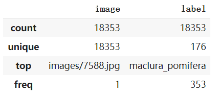 用条形图可视化176类图片的分布(数目)。
 把label标签按字母排个序,这里仅显示前10个。
【本文地址】