| Python图像识别实战(五):卷积神经网络CNN模型图像二分类预测结果评价(附源码和实现效果) | 您所在的位置:网站首页 › 神经网络图像分类代码 › Python图像识别实战(五):卷积神经网络CNN模型图像二分类预测结果评价(附源码和实现效果) |
Python图像识别实战(五):卷积神经网络CNN模型图像二分类预测结果评价(附源码和实现效果)
|
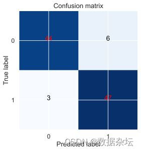
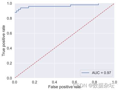
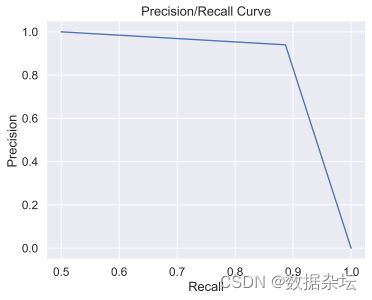
前面我介绍了可视化的一些方法以及机器学习在预测方面的应用,分为分类问题(预测值是离散型)和回归问题(预测值是连续型)(具体见之前的文章)。 从本期开始,我将做一个关于图像识别的系列文章,让读者慢慢理解python进行图像识别的过程、原理和方法,每一篇文章从实现功能、实现代码、实现效果三个方面进行展示。 实现功能: 卷积神经网络CNN模型图像二分类预测结果评价 实现代码: import os from PIL import Image import numpy as np import matplotlib.pyplot as plt import tensorflow as tf from tensorflow.keras import datasets, layers, models from collections import Counter from sklearn.metrics import precision_recall_curve from sklearn.metrics import roc_curve, auc from sklearn.metrics import roc_auc_score import itertools from pylab import mpl import seaborn as sns class Solution(): #==================读取图片================================= def read_image(self,paths): os.listdir(paths) filelist = [] for root, dirs, files in os.walk(paths): for file in files: if os.path.splitext(file)[1] == ".png": filelist.append(os.path.join(root, file)) print(filelist) return filelist #==================图片数据转化为数组========================== def im_array(self,paths): M=[] for filename in paths: im=Image.open(filename) im_L=im.convert("L") #模式L Core=im_L.getdata() arr1=np.array(Core,dtype='float32')/255.0 list_img=arr1.tolist() M.extend(list_img) return M def CNN_model(self,train_images, train_lables): # ============构建卷积神经网络并保存========================= model = models.Sequential() model.add(layers.Conv2D(32, (3, 3), activation='relu', input_shape=(128, 128, 1))) # 过滤器个数,卷积核尺寸,激活函数,输入形状 model.add(layers.MaxPooling2D((2, 2))) # 池化层 model.add(layers.Conv2D(64, (3, 3), activation='relu')) model.add(layers.MaxPooling2D((2, 2))) model.add(layers.Conv2D(64, (3, 3), activation='relu')) model.add(layers.Flatten()) # 降维 model.add(layers.Dense(64, activation='relu')) # 全连接层 model.add(layers.Dense(2, activation='softmax')) # 注意这里参数,我只有两类图片,所以是2. model.summary() # 显示模型的架构 model.compile(optimizer='adam', loss='sparse_categorical_crossentropy', metrics=['accuracy']) return model if __name__=='__main__': Object1=Solution() # =================数据读取=============== path1="D:\DCTDV2\dataset\\train\\" test1 = "D:\DCTDV2\dataset\\test\\" pathDir = os.listdir(path1) print(pathDir) pathDir=pathDir[1:5] print(pathDir) for a in pathDir: path2=path1+a test2=test1+a filelist_1=Object1.read_image(path1+"Norm") filelist_2=Object1.read_image(path2) filelist_all=filelist_1+filelist_2 M=Object1.im_array(filelist_all) train_images=np.array(M).reshape(len(filelist_all),128,128)#输出验证一下(400, 128, 128) label=[0]*len(filelist_1)+[1]*len(filelist_2) train_lables=np.array(label) #数据标签 train_images = train_images[..., np.newaxis] #数据图片 print(train_images.shape)#输出验证一下(400, 128, 128, 1) print(train_lables.shape) # ===================准备测试数据================== filelist_1T = Object1.read_image(test1+"Norm") filelist_2T = Object1.read_image(test2) filelist_allT = filelist_1T + filelist_2T print(filelist_allT) N = Object1.im_array(filelist_allT) dict_label = {0: 'norm', 1: 'IgaK'} test_images = np.array(N).reshape(len(filelist_allT), 128, 128) label = [0] * len(filelist_1T) + [1] * len(filelist_2T) test_lables = np.array(label) # 数据标签 test_images = test_images[..., np.newaxis] # 数据图片 print(test_images.shape) # 输出验证一下(100, 128, 128, 1) print(test_lables.shape) # #===================训练模型============= model=Object1.CNN_model(train_images, train_lables) CnnModel=model.fit(train_images, train_lables, epochs=20) # model.save('D:\电池条带V2\model\my_model.h5') # 保存为h5模型 # tf.keras.models.save_model(model,"F:\python\moxing\model")#这样是pb模型 print("模型保存成功!") # history列表 print(CnnModel.history.keys()) font = {'family': 'Times New Roman','size': 12,} sns.set(font_scale=1.2) plt.plot(CnnModel.history['loss']) plt.title('model loss') plt.ylabel('loss') plt.xlabel('epoch') plt.savefig('D:\\DCTDV2\\result\\V1\\loss' + "\\" + '%s.tif' % a,bbox_inches='tight',dpi=600) plt.show() plt.plot(CnnModel.history['accuracy']) plt.title('model accuracy') plt.ylabel('accuracy') plt.xlabel('epoch') plt.savefig('D:\\DCTDV2\\result\\V1\\accuracy' + "\\" + '%s.tif' % a,bbox_inches='tight',dpi=600) plt.show() # #===================预测图像============= predict_label=[] prob_label=[] for i in test_images: i=np.array([i]) predictions_single=model.predict(i) print(np.argmax(predictions_single)) out_c_1 = np.array(predictions_single)[:, 1] prob_label.extend(out_c_1) predict_label.append(np.argmax(predictions_single)) print(prob_label) print(predict_label) print(list(test_lables)) count = Counter(predict_label) print(count) TP = FP = FN = TN = 0 for i in range(len(predict_label)): if predict_label[i]==1: if list(test_lables)[i]==1: TP=TP+1 elif list(test_lables)[i]==0: FP=FP+1 elif predict_label[i]==0: if list(test_lables)[i]==1: FN=FN+1 elif list(test_lables)[i]==0: TN=TN+1 print(TP,FP,FN,TN) deathc_recall=TP/(TP+FN) savec_recall=TN/(FP+TN) print(deathc_recall) print(savec_recall) print("--------------------") cm = np.arange(4).reshape(2, 2) cm[0, 0] = TN cm[0, 1] = FP cm[1, 0] = FN cm[1, 1] = TP classes = [0, 1] plt.figure() plt.imshow(cm, interpolation='nearest', cmap=plt.cm.Blues) plt.title('Confusion matrix') tick_marks = np.arange(len(classes)) plt.xticks(tick_marks, classes, rotation=0) plt.yticks(tick_marks, classes) thresh = cm.max() / 2. for i, j in itertools.product(range(cm.shape[0]), range(cm.shape[1])): plt.text(j, i, cm[i, j], horizontalalignment="center", color="red" if cm[i, j] > thresh else "black") plt.tight_layout() plt.ylabel('True label') plt.xlabel('Predicted label') plt.savefig('D:\\DCTDV2\\result\\V1\\cm' + "\\" + '%s.tif' % a,bbox_inches='tight',dpi=600) plt.show() fpr, tpr, thresholds = roc_curve(list(test_lables), prob_label, pos_label=1) Auc_score = roc_auc_score(list(test_lables), predict_label) Auc = auc(fpr, tpr) print(Auc_score, Auc) plt.plot(fpr, tpr, 'b', label='AUC = %0.2f' % Auc) # 生成ROC曲线 plt.legend(loc='lower right') plt.plot([0, 1], [0, 1], 'r--') plt.xlim([0, 1]) plt.ylim([0, 1]) plt.ylabel('True positive rate') plt.xlabel('False positive rate') plt.savefig('D:\\DCTDV2\\result\\V1\\roc' + "\\" + '%s.tif' % a,bbox_inches='tight',dpi=600) plt.show() plt.figure() precision, recall, thresholds = precision_recall_curve(list(test_lables), predict_label) plt.title('Precision/Recall Curve') # give plot a title plt.xlabel('Recall') # make axis labels plt.ylabel('Precision') plt.plot(precision, recall) plt.savefig('D:\\DCTDV2\\result\\V1\\pr' + "\\" + '%s.tif' % a,bbox_inches='tight',dpi=600) plt.show()实现效果: 由于数据为非公开数据,仅展示几个图像的效果,有问题可以后台联系我。
本人读研期间发表5篇SCI数据挖掘相关论文,现在在某研究院从事数据挖掘相关工作,对数据挖掘有一定的认知和理解,会不定期分享一些关于python机器学习、深度学习、数据挖掘基础知识与案例。 致力于只做原创,以最简单的方式理解和学习,关注我一起交流成长。 关注V订阅号:数据杂坛可在后台联系我获取相关数据集和源码,送有关数据分析、数据挖掘、机器学习、深度学习相关的电子书籍。 |
【本文地址】
公司简介
联系我们