| TensorFlow 2.0 学习笔记 | 您所在的位置:网站首页 › 神经网络schedule更新参数 › TensorFlow 2.0 学习笔记 |
TensorFlow 2.0 学习笔记
|
第二章 神经网络优化及参数更新
本讲目标:学会神经网络优化过程,使用正则化减少过拟合,使用优化器更新网络参数。 预备知识 神经网络复杂度 指数衰减学习率 激活函数 损失函数 欠拟合与过拟合 正则化减少过拟合 优化器更新网络参数 2.1 预备知识 tf.where()条件语句真返回A,条件语句假返回B tf.where(条件语句, 真返回A, 假返回B) import tensorflow as tf a = tf.constant([1, 2, 3, 1, 1]) b = tf.constant([0, 1, 3, 4, 5]) c = tf.where(tf.greater(a, b), a, b) # 若 a > b, 返回 a 对应位置的元素,否则返回 b 对应的元素 print('c:', c) # 运行结果: # c: tf.Tensor([1 2 3 4 5], shape=(5,), dtype=int32) np.random.RandomState.rand()返回一个 [0, 1) 之间的随机数 np.random.RandomState.rand(维度) # 维度为空,返回标量 import numpy as np rdm = np.random.RandomState(seed=1) # seed 定义生成随机数 a = rdm.rand() # 返回一个标量 b = rdm.rand(2, 3) # 返回维度为2行3列随机数矩阵 print('a:', a) print('b:', b) # 运行结果: # a: 0.417022004702574 # b: [[7.20324493e-01 1.14374817e-04 3.02332573e-01] # [1.46755891e-01 9.23385948e-02 1.86260211e-01]] np.vstack()将两个数组按垂直方向叠加(组合称新的数组) np.vstack(数组1, 数组2) import numpy as np a = np.array([1, 2, 3]) b = np.array([4, 5, 6]) c = np.vstack((a, b)) print('c:', c) # 运行结果: # c: [[1 2 3] # [4 5 6]] np.mgrid[] .ravle() np.c_[]np.mgrid[] [起始值, 结束值) np.mgrid[起始值: 结束值: 步长, 起始值: 结束值: 步长, ...] .ravle() 将x变为一维数组,“把 .前变量拉直” np.c[] 使返回的间隔数值点配对 np.c[数组1, 数组2, ...] import numpy as np import tensorflow as tf # 生成等间隔数值点 x, y = np.mgrid[1:3:1, 2:4:0.5] # 为了保持维度相同,构成网格,故 x, y 都是四列的 # 将x, y拉直,并合并配对为二维张量,生成二维坐标点 grid = np.c_[x.ravel(), y.ravel()] print("x:\n", x) print("y:\n", y) print("x.ravel():\n", x.ravel()) print("y.ravel():\n", y.ravel()) print('grid:\n', grid) # 运行结果 # x: # [[1. 1. 1. 1.] # [2. 2. 2. 2.]] # y: # [[2. 2.5 3. 3.5] # [2. 2.5 3. 3.5]] # x.ravel(): # [1. 1. 1. 1. 2. 2. 2. 2.] # y.ravel(): # [2. 2.5 3. 3.5 2. 2.5 3. 3.5] # grid: # [[1. 2. ] # [1. 2.5] # [1. 3. ] # [1. 3.5] # [2. 2. ] # [2. 2.5] # [2. 3. ] # [2. 3.5]] 2.2 复杂度学习率 神经网络的复杂度NN复杂度:多用NN层数和NN参数的个数表示
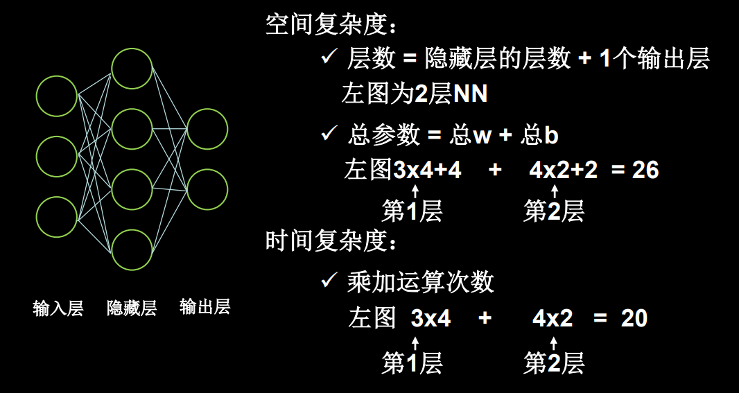
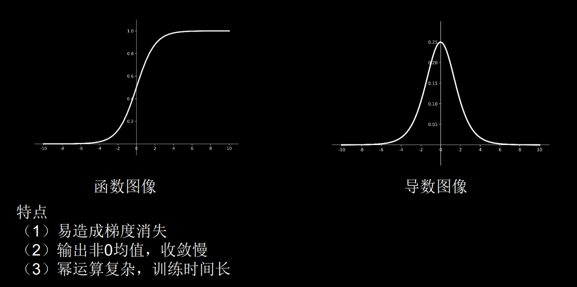
空间复杂度: ✅ 层数 = 隐藏层的层数 + 1个输出层 上图为2层NN ✅总参数 = 总w + 总b 上图为3 * 4 + 4 + 4 * 2 + 2 = 26 时间复杂度: ✅乘加运算次数 上图 3 * 4 + 4 * 2 = 20 学习率学习率lr=0.001过慢, lr=0.999不收敛 指数衰减学习率 可以先用较大的学习率,快速得到较优解,然后逐步减小学习率,使模型在训练后期稳定。 指数衰减学习率 = 初始学习率 * 学习衰减率 ^ (当前轮数 / 多少轮衰减一次) epoch = 40 LR_BASE = 0.2 LRDECAY = 0.99 LR_STEP = 1 for epoch in range(epoch): lr = LR_BASE * LR_DECAY ** (epoch / LR_STEP) # 指数衰减 with tf.GradientTape() as tape: loss = tf.square(w + 1) grads = tape.gradient(loss, w) w.assign_sub(lr * grads) print("After %s epoch,w is %f,loss is %f, lr is %f" % (epoch, w.numpy(), loss, lr)) # 运行结果 # After 33 epoch,w is -0.999996,loss is 0.000000,lr is 0.143546 # After 34 epoch,w is -0.999997,loss is 0.000000,lr is 0.142111 # After 35 epoch,w is -0.999998,loss is 0.000000,lr is 0.140690 # After 36 epoch,w is -0.999999,loss is 0.000000,lr is 0.139283 # After 37 epoch,w is -0.999999,loss is 0.000000,lr is 0.137890 # After 38 epoch,w is -0.999999,loss is 0.000000,lr is 0.136511 # After 39 epoch,w is -0.999999,loss is 0.000000,lr is 0.135146 2.3 激活函数Sigmoid函数 \[f(x)=\frac{1}{1+e^{-x}} \]tf.nn.sigmoid(x) # 将输入值变换到 (0, 1) 之间输出 特点: (1)易造成梯度消失 (2)输出非0均值,收敛慢 (3)幂运算复杂,训练时间长
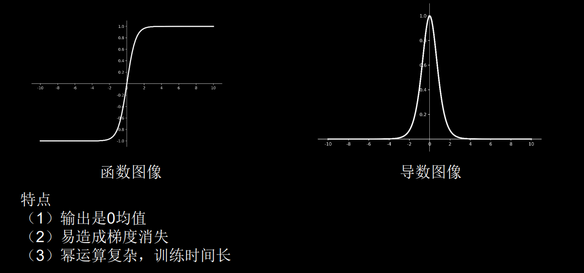
Tanh函数 \[f(x)=\frac{1-e^{-2x}}{1+e^{-2x}} \]tf.math.tanh(x) 特点: (1)输出是0均值 (2)易造成梯度消失 (3)幂运算复杂,训练时间长
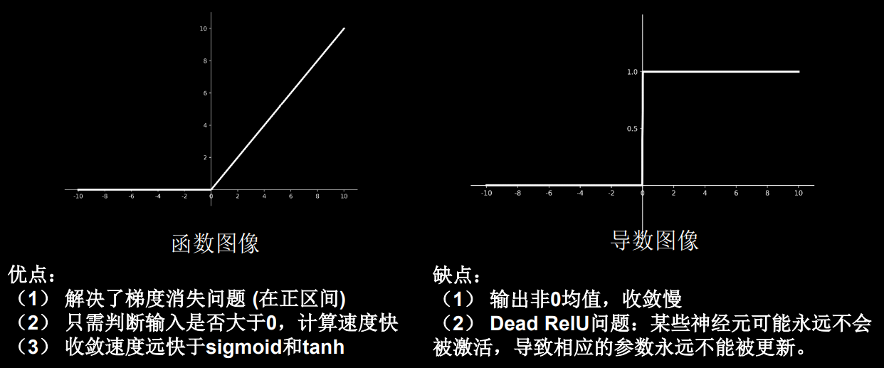
Relu函数 \[f(x)=max(x, 0)= \]tf.nn.relu(x) 优点: (1)解决了梯度消失问题(在正区间) (2)只需判断输入是否大于0,计算速度快 (3)收敛速度远快于sigmoid和tanh 缺点: (1)输出非0均值,收敛慢 (2)Dead ReIU问题:某些神经元可能永远不会被激活,导致相应的参数永远不能被更新。
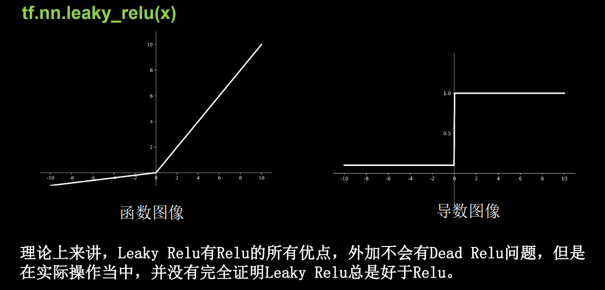
Leaky Relu tf.nn.leaky_relu(x) 特点: 理论上来讲,Leaky Relu有Relu的所有优点,外加不会有Dead Relu问题,但是在实际操作当中,并没有完全证明Leaky Relu总是好于Relu。
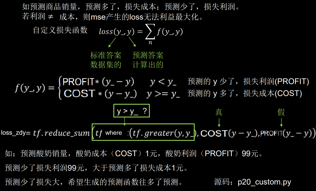
对于初学者的建议 首选relu激活函数 学习率设置较小值 输入特征标准化,即让输入特征满足以0为均值,1为标准差的正态分布 初始参数中心化,即让随机生成的参数满足以0为均值,\(\sqrt{\frac{2}{当前输入特征个数}}\) 为标准差的正态分布。 2.4 损失函数损失函数 (loss): 预测值 (y) 与已知答案 (y_) 的差距 NN优化目标: loss最小 mse(Mean Squared Error) 自定义 ce(Cross Entropy) # 交叉熵均方误差 mse \[MSE({y_\_},y)=\frac{\sum_{i=1}^n (y - y_\_)^2}{n} \]loss_mse = tf.reduce_mean(tf.square(y_ - y))💬 Example 预测酸奶日销量y,x1,x2是影响日销量的因素。 建模前,应预先采集的数据有:每日x1、x2和销量y_(即已知答案,最佳情况:产量=销量) 拟造数据集X, Y_: y_ = x1 + x2 噪声:-0.05~+0.05 拟合可以预测销量的函数 import tensorflow as tf import numpy as np SEED = 23455 rdm = np.random.RandomState(seed=SEED) # 生成[0,1)之间的随机数 x = rdm.rand(32, 2) # 32行两列的 [0, 1) 之间的随机数 y_ = [[x1 + x2 + (rdm.rand() / 10.0 - 0.05)] for (x1, x2) in x] # 生成噪声[0,1)/10=[0,0.1); [0,0.1)-0.05=[-0.05,0.05) x = tf.cast(x, dtype=tf.float32) w1 = tf.Variable(tf.random.normal([2, 1], stddev=1, seed=1)) epoch = 15000 lr = 0.002 for epoch in range(epoch): with tf.GradientTape() as tape: y = tf.matmul(x, w1) loss_mse = tf.reduce_mean(tf.square(y_ - y)) grads = tape.gradient(loss_mse, w1) w1.assign_sub(lr * grads) if epoch % 500 == 0: print("After %d training steps,w1 is " % (epoch)) print(w1.numpy(), "\n") print("Final w1 is: ", w1.numpy()) # 运行结果 # After 14500 training steps,w1 is # [[1.0002553 ] # [0.99838644]] # # Final w1 is: [[1.0009792] # [0.9977485]]自定义损失函数: 如预测商品销量,预测多了,损失成本,预测少了,损失利润。 若利润 ≠ 成本,则 mse 产生的 loss 无法利益最大化 自定义损失函数 \(loss(y_\_,y)=\sum_{n}{f(y_\_,y)}\)
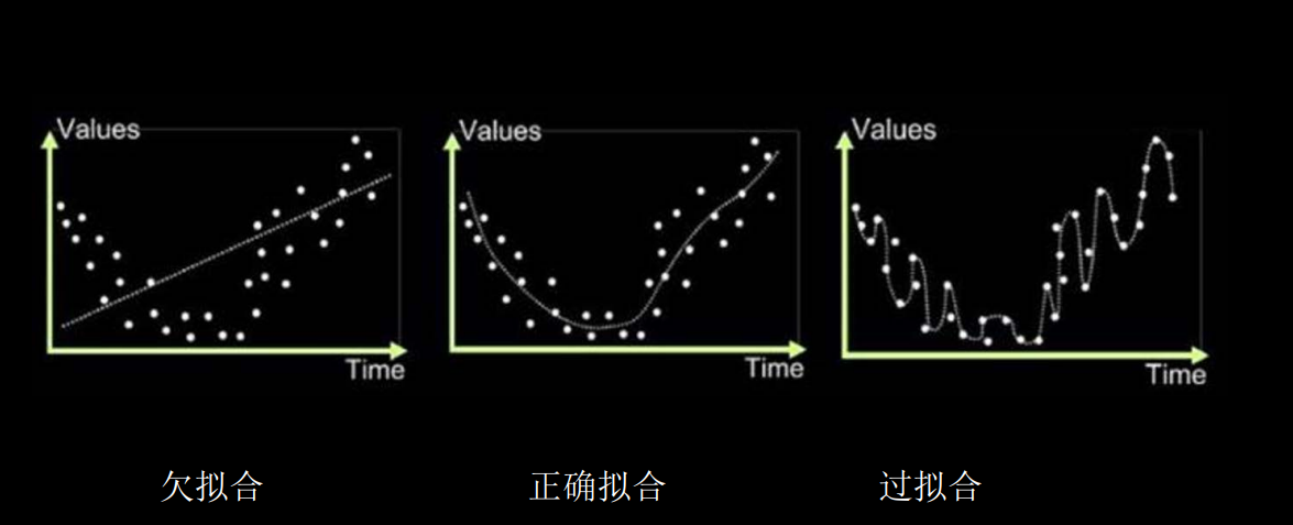
交叉熵损失函数 CE (Cross Entropy): 表征两个概率分布之间的距离 \[H(y_\_,y)=-\sum{y_\_*\ln y} \]eg. 二分类已知答案 y_ = (1, 0) 预测 y1=(0.6, 0.5) y2 = (0.8, 0.2), 哪个更接近标准答案? \[H_1((1, 0), (0.6, 0.4)) = -(1 * \ln0.6 + 0 * \ln0.4)\approx -(-0.511 +0)=0.511\\ H_2((1, 0), (0.8, 0.2)) = -(1 * \ln0.8 + 0 * \ln0.2)\approx -(-0.223 +0)=0.223 \]因为 H1 > H2,所以 y2 预测更准 tf.losses.categorical_crossentropy(y_, y) import tensorflow as tf loss_ce1 = tf.losses.categorical_crossentropy([1, 0], [0.6, 0.4]) loss_ce2 = tf.losses.categorical_crossentropy([1, 0], [0.8, 0.2]) print("loss_ce1:", loss_ce1) print("loss_ce2:", loss_ce2) # 交叉熵损失函数 # 运行结果 # loss_ce1: tf.Tensor(0.5108256, shape=(), dtype=float32) # loss_ce2: tf.Tensor(0.22314353, shape=(), dtype=float32)softmax 与交叉熵结合 输出先过softmax函数,再计算y与y_的交叉熵损失函数 tf.nn.softmax_cross_entropy_with_logits(y_, y) # softmax与交叉熵损失函数的结合 import tensorflow as tf import numpy as np y_ = np.array([[1, 0, 0], [0, 1, 0], [0, 0, 1], [1, 0, 0], [0, 1, 0]]) y = np.array([[12, 3, 2], [3, 10, 1], [1, 2, 5], [4, 6.5, 1.2], [3, 6, 1]]) y_pro = tf.nn.softmax(y) loss_ce1 = tf.losses.categorical_crossentropy(y_,y_pro) loss_ce2 = tf.nn.softmax_cross_entropy_with_logits(y_, y) print('分步计算的结果:\n', loss_ce1) print('结合计算的结果:\n', loss_ce2) # 输出的结果相同 # 运行结果 # 分步计算的结果: # tf.Tensor( # [1.68795487e-04 1.03475622e-03 6.58839038e-02 2.58349207e+00 # 5.49852354e-02], shape=(5,), dtype=float64) # 结合计算的结果: # tf.Tensor( # [1.68795487e-04 1.03475622e-03 6.58839038e-02 2.58349207e+00 # 5.49852354e-02], shape=(5,), dtype=float64) 2.5 缓解过拟合欠拟合与过拟合
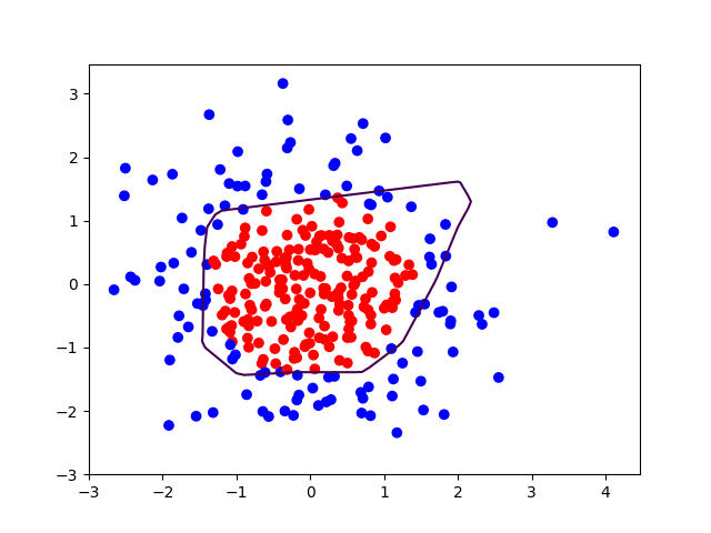
欠拟合的解决方法: 增加输入特征项 增加网络参数 减少正则化参数过拟合的解决方法: 数据清洗 增大训练集 采用正则化 增大正则化参数正则化缓解过拟合 正则化在损失函数中引入模型复杂度指标,利用给W加权值,弱化了训练数据的噪声(一般不正则化b) loss = loss(y, y_) + REGULARIZER * loss(w) loss(y, y_)模型中所有参数的损失函数如:交叉熵、均方误差 REGULARIZER用超参数REGULARIZER给出参数w在总loss中的比例,即正则化的权重 loss(w)需要正则化的参数 loss(w)包括两种正则化: L1正则化 \(loss_{L1}(w)=\sum_i \lvert w_i \rvert\) L2正则化 \(loss_{L2}(w)=\sum_i \lvert w_i^2 \rvert\) 正则化的选择 L1正则化大概率会使很多参数变为零,因此该方法可通过稀疏参数,即减少参数的数量,降低复杂度。 L2正则化会使参数很接近零但不为零,因此该方法可通过减小参数的值的大小降低复杂度。 正则化缓解过拟合 with tf.GradientTape() as tape: # 记录梯度信息 h1 = tf.matmul(x_train, w1) + b1 # 记录神经网络乘加运算 h1 = tf.nn.relu(h1) y = tf.matmul(h1, w2) + b2 # 采用均方误差损失函数mse = mean(sum(y-out)^2) loss_mse = tf.reduce_mean(tf.square(y_train - y)) # 添加l2正则化 loss_regularization = [] # tf.nn.l2_loss(w)=sum(w ** 2) / 2 loss_regularization.append(tf.nn.l2_loss(w1)) loss_regularization.append(tf.nn.l2_loss(w2)) # 求和 # 例:x=tf.constant(([1,1,1],[1,1,1])) # tf.reduce_sum(x) # >>>6 loss_regularization = tf.reduce_sum(loss_regularization) loss = loss_mse + 0.03 * loss_regularization # REGULARIZER = 0.03 Variable = [w1, b1, w2, b2] grads = tape.gradient(loss, variables)example 实例 x1 x2 y_c -0.416757847 -0.056266827 1 -2.136196096 1.640270808 0 -1.793435585 -0.841747366 0 0.502881417 -1.245288087 1 -1.057952219 -0.909007615 1 0.551454045 2.292208013 0 0.041539393 -1.117925445 1 0.539058321 -0.5961597 1 -0.019130497 1.17500122 1 0.0380472 -0.21714 ? # 导入所需模块 import tensorflow as tf from matplotlib import pyplot as plt import numpy as np import pandas as pd # 读入数据/标签 生成x_train y_train df = pd.read_csv('dot.csv') x_data = np.array(df[['x1', 'x2']]) y_data = np.array(df['y_c']) x_train = np.vstack(x_data).reshape(-1, 2) y_train = np.vstack(y_data).reshape(-1, 1) Y_c = [['red' if y else 'blue'] for y in y_train] # 转换x的数据类型,否则后面矩阵相乘时会因数据类型问题报错 x_train = tf.cast(x_train, tf.float32) y_train = tf.cast(y_train, tf.float32) # from_tensor_slices函数切分传入的张量的第一个维度,生成相应的数据集,使输入特征和标签值一一对应 train_db = tf.data.Dataset.from_tensor_slices((x_train, y_train)).batch(32) # 生成神经网络的参数,输入层为2个神经元,隐藏层为11个神经元(自己随机选择的),1层隐藏层,输出层为1个神经元 # 用tf.Variable()保证参数可训练 w1 = tf.Variable(tf.random.normal([2, 11]), dtype=tf.float32) b1 = tf.Variable(tf.constant(0.01, shape=[11])) w2 = tf.Variable(tf.random.normal([11, 1]), dtype=tf.float32) b2 = tf.Variable(tf.constant(0.01, shape=[1])) lr = 0.01 # 学习率 epoch = 400 # 循环轮数 # 训练部分 for epoch in range(epoch): for step, (x_train, y_train) in enumerate(train_db): with tf.GradientTape() as tape: # 记录梯度信息 h1 = tf.matmul(x_train, w1) + b1 # 记录神经网络乘加运算 h1 = tf.nn.relu(h1) y = tf.matmul(h1, w2) + b2 # 采用均方误差损失函数mse = mean(sum(y-out)^2) loss = tf.reduce_mean(tf.square(y_train - y)) # 计算loss对各个参数的梯度 variables = [w1, b1, w2, b2] grads = tape.gradient(loss, variables) # 实现梯度更新 # w1 = w1 - lr * w1_grad tape.gradient是自动求导结果与[w1, b1, w2, b2] 索引为0,1,2,3 w1.assign_sub(lr * grads[0]) b1.assign_sub(lr * grads[1]) w2.assign_sub(lr * grads[2]) b2.assign_sub(lr * grads[3]) # 每20个epoch,打印loss信息 if epoch % 20 == 0: print('epoch:', epoch, 'loss:', float(loss)) # 预测部分 print("*******predict*******") # xx在-3到3之间以步长为0.01,yy在-3到3之间以步长0.01,生成间隔数值点 xx, yy = np.mgrid[-3:3:.1, -3:3:.1] # 将xx , yy拉直,并合并配对为二维张量,生成二维坐标点 grid = np.c_[xx.ravel(), yy.ravel()] grid = tf.cast(grid, tf.float32) # 将网格坐标点喂入神经网络,进行预测,probs为输出 probs = [] for x_test in grid: # 使用训练好的参数进行预测 h1 = tf.matmul([x_test], w1) + b1 h1 = tf.nn.relu(h1) y = tf.matmul(h1, w2) + b2 # y为预测结果 probs.append(y) # 取第0列给x1,取第1列给x2 x1 = x_data[:, 0] x2 = x_data[:, 1] # probs的shape调整成xx的样子 probs = np.array(probs).reshape(xx.shape) plt.scatter(x1, x2, color=np.squeeze(Y_c)) #squeeze去掉纬度是1的纬度,相当于去掉[['red'],[''blue]],内层括号变为['red','blue'] # 把坐标xx yy和对应的值probs放入contour函数,给probs值为0.5的所有点上色 plt点show后 显示的是红蓝点的分界线 plt.contour(xx, yy, probs, levels=[.5]) plt.show() # 读入红蓝点,画出分割线,不包含正则化 # 不清楚的数据,建议print出来查看 # 运行结果 # epoch: 360 loss: 0.01718108169734478 # epoch: 380 loss: 0.017415596172213554
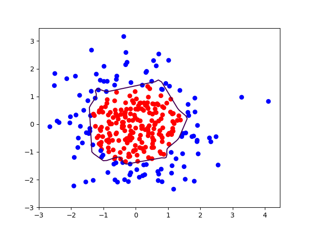
曲线不平滑,存在过拟合。 下面改进 # 导入所需模块 import tensorflow as tf from matplotlib import pyplot as plt import numpy as np import pandas as pd # 读入数据/标签 生成x_train y_train df = pd.read_csv('dot.csv') x_data = np.array(df[['x1', 'x2']]) y_data = np.array(df['y_c']) x_train = x_data y_train = y_data.reshape(-1, 1) Y_c = [['red' if y else 'blue'] for y in y_train] # 转换x的数据类型,否则后面矩阵相乘时会因数据类型问题报错 x_train = tf.cast(x_train, tf.float32) y_train = tf.cast(y_train, tf.float32) # from_tensor_slices函数切分传入的张量的第一个维度,生成相应的数据集,使输入特征和标签值一一对应 train_db = tf.data.Dataset.from_tensor_slices((x_train, y_train)).batch(32) # 生成神经网络的参数,输入层为4个神经元,隐藏层为32个神经元,2层隐藏层,输出层为3个神经元 # 用tf.Variable()保证参数可训练 w1 = tf.Variable(tf.random.normal([2, 11]), dtype=tf.float32) b1 = tf.Variable(tf.constant(0.01, shape=[11])) w2 = tf.Variable(tf.random.normal([11, 1]), dtype=tf.float32) b2 = tf.Variable(tf.constant(0.01, shape=[1])) lr = 0.01 # 学习率为 epoch = 400 # 循环轮数 # 训练部分 for epoch in range(epoch): for step, (x_train, y_train) in enumerate(train_db): with tf.GradientTape() as tape: # 记录梯度信息 h1 = tf.matmul(x_train, w1) + b1 # 记录神经网络乘加运算 h1 = tf.nn.relu(h1) y = tf.matmul(h1, w2) + b2 # 采用均方误差损失函数mse = mean(sum(y-out)^2) loss_mse = tf.reduce_mean(tf.square(y_train - y)) # 添加l2正则化 loss_regularization = [] # tf.nn.l2_loss(w)=sum(w ** 2) / 2 loss_regularization.append(tf.nn.l2_loss(w1)) loss_regularization.append(tf.nn.l2_loss(w2)) # 求和 # 例:x=tf.constant(([1,1,1],[1,1,1])) # tf.reduce_sum(x) # >>>6 # loss_regularization = tf.reduce_sum(tf.stack(loss_regularization)) loss_regularization = tf.reduce_sum(loss_regularization) loss = loss_mse + 0.03 * loss_regularization #REGULARIZER = 0.03 # 计算loss对各个参数的梯度 variables = [w1, b1, w2, b2] grads = tape.gradient(loss, variables) # 实现梯度更新 # w1 = w1 - lr * w1_grad w1.assign_sub(lr * grads[0]) b1.assign_sub(lr * grads[1]) w2.assign_sub(lr * grads[2]) b2.assign_sub(lr * grads[3]) # 每200个epoch,打印loss信息 if epoch % 20 == 0: print('epoch:', epoch, 'loss:', float(loss)) # 预测部分 print("*******predict*******") # xx在-3到3之间以步长为0.01,yy在-3到3之间以步长0.01,生成间隔数值点 xx, yy = np.mgrid[-3:3:.1, -3:3:.1] # 将xx, yy拉直,并合并配对为二维张量,生成二维坐标点 grid = np.c_[xx.ravel(), yy.ravel()] grid = tf.cast(grid, tf.float32) # 将网格坐标点喂入神经网络,进行预测,probs为输出 probs = [] for x_predict in grid: # 使用训练好的参数进行预测 h1 = tf.matmul([x_predict], w1) + b1 h1 = tf.nn.relu(h1) y = tf.matmul(h1, w2) + b2 # y为预测结果 probs.append(y) # 取第0列给x1,取第1列给x2 x1 = x_data[:, 0] x2 = x_data[:, 1] # probs的shape调整成xx的样子 probs = np.array(probs).reshape(xx.shape) plt.scatter(x1, x2, color=np.squeeze(Y_c)) # 把坐标xx yy和对应的值probs放入contour函数,给probs值为0.5的所有点上色 plt点show后 显示的是红蓝点的分界线 plt.contour(xx, yy, probs, levels=[.5]) plt.show() # 读入红蓝点,画出分割线,包含正则化 # 不清楚的数据,建议print出来查看 # 运行结果 # epoch: 340 loss: 0.10149043053388596 # epoch: 360 loss: 0.09740603715181351 # epoch: 380 loss: 0.09389346837997437
相对平滑,缓解过拟合。 2.6 优化器 神经网络参数优化器待优化参数w,损失函数loss,学习率lr,每次迭代一个batch,t 表示当前batch迭代的总次数:(每个batch通常包含2的n次方个数) 计算 t 时刻损失函数关于当前参数的梯度 $ g_t=\nabla loss = \frac{\partial loss}{\partial (w_t)} $ 计算 t 时刻一阶动量 \(m_t\) 和二阶动量 \(V_t\) 计算 t 时刻下降梯度:\(\eta_t = lr * m_t / \sqrt{V_t}\) 计算 t + 1 时刻参数:\(w_{t+1} = w_t - \eta _t = w_t - lr * m_t / \sqrt{V_t}\)一阶动量:与梯度相关的函数 二阶动量:与梯度平方相关的函数 优化器SGD(无 momentum),常用的梯度下降法。(不含动量) \(m_t = g_t \ \ \ \ \ \ \ \ V_t = 1\) \(\eta _t = lr * m_t / \sqrt{V_t} = lr * g_t\) \(w_{t+1} = w_t - \eta _t = w_t - lr * m_t / \sqrt{V_t} = w_t -lr * g_t\) \(w_{t+1} = w_t - lr * \frac {\partial loss} {\partial w_t}\) # SGD 单层网络 w1.assign_sub(lr * grads[0]) # 参数w1自更新 b1.assign_sub(lr * grads[1]) # 参数b1自更新 # 利用鸢尾花数据集,实现前向传播、反向传播,可视化loss曲线 # 导入所需模块 import tensorflow as tf from sklearn import datasets from matplotlib import pyplot as plt import numpy as np import time ##1## 引入时间模块,可以对比不同优化器运行时间 # 导入数据,分别为输入特征和标签 x_data = datasets.load_iris().data y_data = datasets.load_iris().target # 随机打乱数据(因为原始数据是顺序的,顺序不打乱会影响准确率) # seed: 随机数种子,是一个整数,当设置之后,每次生成的随机数都一样(为方便教学,以保每位同学结果一致) np.random.seed(116) # 使用相同的seed,保证输入特征和标签一一对应 np.random.shuffle(x_data) np.random.seed(116) np.random.shuffle(y_data) tf.random.set_seed(116) # 将打乱后的数据集分割为训练集和测试集,训练集为前120行,测试集为后30行 x_train = x_data[:-30] y_train = y_data[:-30] x_test = x_data[-30:] y_test = y_data[-30:] # 转换x的数据类型,否则后面矩阵相乘时会因数据类型不一致报错 x_train = tf.cast(x_train, tf.float32) x_test = tf.cast(x_test, tf.float32) # from_tensor_slices函数使输入特征和标签值一一对应。(把数据集分批次,每个批次batch组数据) train_db = tf.data.Dataset.from_tensor_slices((x_train, y_train)).batch(32) test_db = tf.data.Dataset.from_tensor_slices((x_test, y_test)).batch(32) # 生成神经网络的参数,4个输入特征故,输入层为4个输入节点;因为3分类,故输出层为3个神经元 # 用tf.Variable()标记参数可训练 # 使用seed使每次生成的随机数相同(方便教学,使大家结果都一致,在现实使用时不写seed) w1 = tf.Variable(tf.random.truncated_normal([4, 3], stddev=0.1, seed=1)) b1 = tf.Variable(tf.random.truncated_normal([3], stddev=0.1, seed=1)) lr = 0.1 # 学习率为0.1 train_loss_results = [] # 将每轮的loss记录在此列表中,为后续画loss曲线提供数据 test_acc = [] # 将每轮的acc记录在此列表中,为后续画acc曲线提供数据 epoch = 500 # 循环500轮 loss_all = 0 # 每轮分4个step,loss_all记录四个step生成的4个loss的和 # 训练部分 now_time = time.time() ##2## for epoch in range(epoch): # 数据集级别的循环,每个epoch循环一次数据集 for step, (x_train, y_train) in enumerate(train_db): # batch级别的循环 ,每个step循环一个batch with tf.GradientTape() as tape: # with结构记录梯度信息 y = tf.matmul(x_train, w1) + b1 # 神经网络乘加运算 y = tf.nn.softmax(y) # 使输出y符合概率分布(此操作后与独热码同量级,可相减求loss) y_ = tf.one_hot(y_train, depth=3) # 将标签值转换为独热码格式,方便计算loss和accuracy loss = tf.reduce_mean(tf.square(y_ - y)) # 采用均方误差损失函数mse = mean(sum(y-out)^2) loss_all += loss.numpy() # 将每个step计算出的loss累加,为后续求loss平均值提供数据,这样计算的loss更准确 # 计算loss对各个参数的梯度 grads = tape.gradient(loss, [w1, b1]) # 实现梯度更新 w1 = w1 - lr * w1_grad b = b - lr * b_grad w1.assign_sub(lr * grads[0]) # 参数w1自更新 b1.assign_sub(lr * grads[1]) # 参数b自更新 # 每个epoch,打印loss信息 print("Epoch {}, loss: {}".format(epoch, loss_all / 4)) train_loss_results.append(loss_all / 4) # 将4个step的loss求平均记录在此变量中 loss_all = 0 # loss_all归零,为记录下一个epoch的loss做准备 # 测试部分 # total_correct为预测对的样本个数, total_number为测试的总样本数,将这两个变量都初始化为0 total_correct, total_number = 0, 0 for x_test, y_test in test_db: # 使用更新后的参数进行预测 y = tf.matmul(x_test, w1) + b1 y = tf.nn.softmax(y) pred = tf.argmax(y, axis=1) # 返回y中最大值的索引,即预测的分类 # 将pred转换为y_test的数据类型 pred = tf.cast(pred, dtype=y_test.dtype) # 若分类正确,则correct=1,否则为0,将bool型的结果转换为int型 correct = tf.cast(tf.equal(pred, y_test), dtype=tf.int32) # 将每个batch的correct数加起来 correct = tf.reduce_sum(correct) # 将所有batch中的correct数加起来 total_correct += int(correct) # total_number为测试的总样本数,也就是x_test的行数,shape[0]返回变量的行数 total_number += x_test.shape[0] # 总的准确率等于total_correct/total_number acc = total_correct / total_number test_acc.append(acc) print("Test_acc:", acc) print("--------------------------") total_time = time.time() - now_time ##3## print("total_time", total_time) ##4## # 绘制 loss 曲线 plt.title('Loss Function Curve') # 图片标题 plt.xlabel('Epoch') # x轴变量名称 plt.ylabel('Loss') # y轴变量名称 plt.plot(train_loss_results, label="$Loss$") # 逐点画出trian_loss_results值并连线,连线图标是Loss plt.legend() # 画出曲线图标 plt.show() # 画出图像 # 绘制 Accuracy 曲线 plt.title('Acc Curve') # 图片标题 plt.xlabel('Epoch') # x轴变量名称 plt.ylabel('Acc') # y轴变量名称 plt.plot(test_acc, label="$Accuracy$") # 逐点画出test_acc值并连线,连线图标是Accuracy plt.legend() plt.show() # 本文件较 class1\p45_iris.py 仅添加四处时间记录 用 ##n## 标识 # 运行结果 # Epoch 497, loss: 0.03235237207263708 # Test_acc: 1.0 # -------------------------- # Epoch 498, loss: 0.03232626663520932 # Test_acc: 1.0 # -------------------------- # Epoch 499, loss: 0.032300274819135666 # Test_acc: 1.0 # -------------------------- # total_time 7.877314805984497SGDM(含momentum的SGD),在SGD基础上增加一阶动量。 \(m_t = \beta * m_{t-1} + (1-\beta)*g_t \ \ \ \ \ \ \ \ V_T = 1\) \(\eta _t = lr * m_t / \sqrt{V_t} = lr * m_t = lr*(\beta*m_{t-1}+(1-\beta)*g_t)\) \(w_{t+1} = w_t - \eta _t = w_t - lr * (\beta*m_{t-1}+(1-\beta)*g_t\) \(m_t = \beta * m_{t-1} + (1-\beta)*g_t \ \ \ \ \ \ \ \ V_t = 1\) # 与SGD不同之处 m_w, m_b = 0, 0 beta = 0.9 # sgd-momentum m_w = beta * m_w + (1 - beta) * grads[0] m_b = beta * m_b + (1 - beta) * grads[1] w1.assign_sub(lr * m_w) b1.assign_sub(lr * m_b) # 运行结果: # -------------------------- # Epoch 498, loss: 0.03065542411059141 # -------------------------- # Epoch 499, loss: 0.030630568508058786 # Test_acc: 1.0 # -------------------------- # total_time 10.623216390609741Adagrad,在SGD基础上增加二阶动量(二阶动量,从开始到现在,梯度平方的累计和) \[m_t = g_t \ \ \ \ \ \ \ V_t =\sum_{\tau=1}^t g_\tau ^2 \]\(\eta_t = lr * m_t / (\sqrt{V_t})=lr*g_t / (\sqrt{\sum_{\tau=1}^t g_\tau ^2})\) \[w_{t+1} = w_t - \eta_t = w_t - lr * g_t/ (\sqrt{\sum_{\tau=1}^t g_\tau ^2}) \]# 与SGD不同之处: v_w, v_b = 0, 0 # adagrad v_w += tf.square(grads[0]) v_b += tf.square(grads[1]) w1.assign_sub(lr * grads[0] / tf.sqrt(v_w)) b1.assign_sub(lr * grads[1] / tf.sqrt(v_b)) # 运行结果: # -------------------------- # Epoch 498, loss: 0.03176002576947212 # Test_acc: 1.0 # -------------------------- # Epoch 499, loss: 0.03173917159438133 # Test_acc: 1.0 # -------------------------- # total_time 7.388378620147705RMSProp,SGD基础上增加二阶动量 \[m_t = g_t \ \ \ \ \ \ \ V_t =\beta * V_{t-1}+(1-\beta)*g_t ^2 \]\(\eta_t = lr * m_t / (\sqrt{V_t})=lr*g_t / (\sqrt{\beta * V_{t-1}+(1-\beta)*g_t ^2})\) \[w_{t+1} = w_t - \eta_t = w_t - lr * g_t/ (\sqrt{\beta * V_{t-1}+(1-\beta)*g_t ^2}) \]# 与SGD不同之处 v_w, v_b = 0, 0 beta = 0.9 # rmsprop v_w = beta * v_w + (1 - beta) * tf.square(grads[0]) v_b = beta * v_b + (1 - beta) * tf.square(grads[1]) w1.assign_sub(lr * grads[0] / tf.sqrt(v_w)) b1.assign_sub(lr * grads[1] / tf.sqrt(v_b)) # 运行结果: # -------------------------- # Epoch 498, loss: nan # Test_acc: 0.36666666666666664 # -------------------------- # Epoch 499, loss: nan # Test_acc: 0.36666666666666664 # -------------------------- # total_time 12.019102573394775Adam,同时结合SGDM一阶动量和RMSProp二阶动量 \(m_t = \beta_1*m_{t-1}+(1-\beta_1)*g_t\) 修正一阶动量的偏差:\(\hat{m_t}=\frac{m_t}{1-\beta_t}\) \(V_t=\beta_2*V_{step-1}+(1-\beta_2)*g_t ^2\) 修正二阶动量的偏差:\(\hat{V_t}=\frac {V_t}{1-\beta_2 ^t}\) \(\eta_t = lr *\hat{m_t}/\sqrt{\hat{V_t}}=lr*\frac{m_t}{1-\beta_1 ^t} / \sqrt{\frac{V_t}{1-\beta_2 ^t}}\) \(w_{t+1} = w_t - \eta_t = w_t-lr*\frac{m_t}{1-\beta_1^t}/ \sqrt{\frac{V_t}{1-\beta_2 ^t}}\) # 与SGD不同之处 m_w, m_b = 0, 0 v_w, v_b = 0, 0 beta1, beta2 = 0.9, 0.999 delta_w, delta_b = 0, 0 global_step = 0 # 后面 +1 # adam m_w = beta1 * m_w + (1 - beta1) * grads[0] m_b = beta1 * m_b + (1 - beta1) * grads[1] v_w = beta2 * v_w + (1 - beta2) * tf.square(grads[0]) v_b = beta2 * v_b + (1 - beta2) * tf.square(grads[1]) m_w_correction = m_w / (1 - tf.pow(beta1, int(global_step))) m_b_correction = m_b / (1 - tf.pow(beta1, int(global_step))) v_w_correction = v_w / (1 - tf.pow(beta2, int(global_step))) v_b_correction = v_b / (1 - tf.pow(beta2, int(global_step))) w1.assign_sub(lr * m_w_correction / tf.sqrt(v_w_correction)) b1.assign_sub(lr * m_b_correction / tf.sqrt(v_b_correction)) # 运行结果: # -------------------------- # Epoch 498, loss: 0.013929554144851863 # Test_acc: 1.0 # -------------------------- # Epoch 499, loss: 0.013926223502494395 # Test_acc: 1.0 # -------------------------- # total_time 8.114784002304077 |
【本文地址】