| Seaborn数据可视化 | 您所在的位置:网站首页 › 数据可视化分析报告总结怎么写 › Seaborn数据可视化 |
Seaborn数据可视化
|
系列文章目录
第一章 探索性数据分析之Seaborn数据可视化 文章目录 系列文章目录前言一、Seaborn简介二、准备阶段1.导入依赖包2.读入数据3.设置样式 三、绘图操作1.线性图2.条形图、热力图3.散点图4.分布图 五.Seaborn后续补充1.seaborn.pairplot 总结 前言本文详细简介的记录了利用Seaborn进行可视化操作,数据可视化是数据分析中重要的一步,在前期数据的探索性分析,以及后期结果的呈现中都有着重要地位。更加全面的教学可进入Kaggle Seaborn教学进行学习。 一、Seaborn简介Python有很多非常优秀易用的数据可视化的库,其中最著名的要数matplotlib了,它有着十几年的历史,至今仍然是Python使用者最常用的画图库。 Seaborn跟matplotlib最大的区别就是它的默认绘图风格和色彩搭配都具有现代美感,其实是在matplotlib的基础上进行了更高级的API封装,让我们能用更少的代码去调用 matplotlib的方法,从而使得作图更加容易,在大多数情况下使用seaborn就能做出很具有吸引力的图,而使用matplotlib就能制作具有更多特色的图。应该把Seaborn视为matplotlib的补充,而不是替代物。 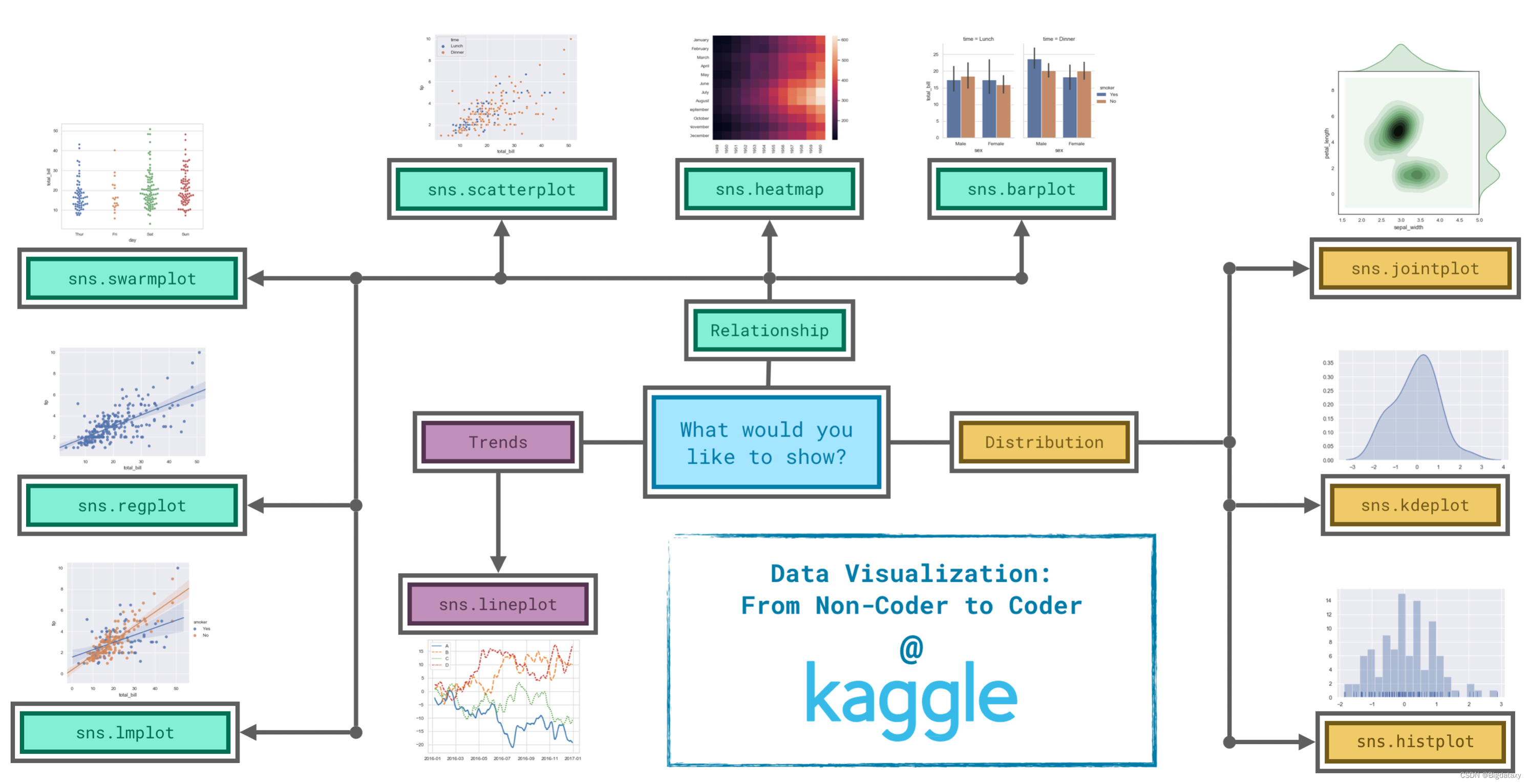 二、准备阶段
1.导入依赖包
二、准备阶段
1.导入依赖包
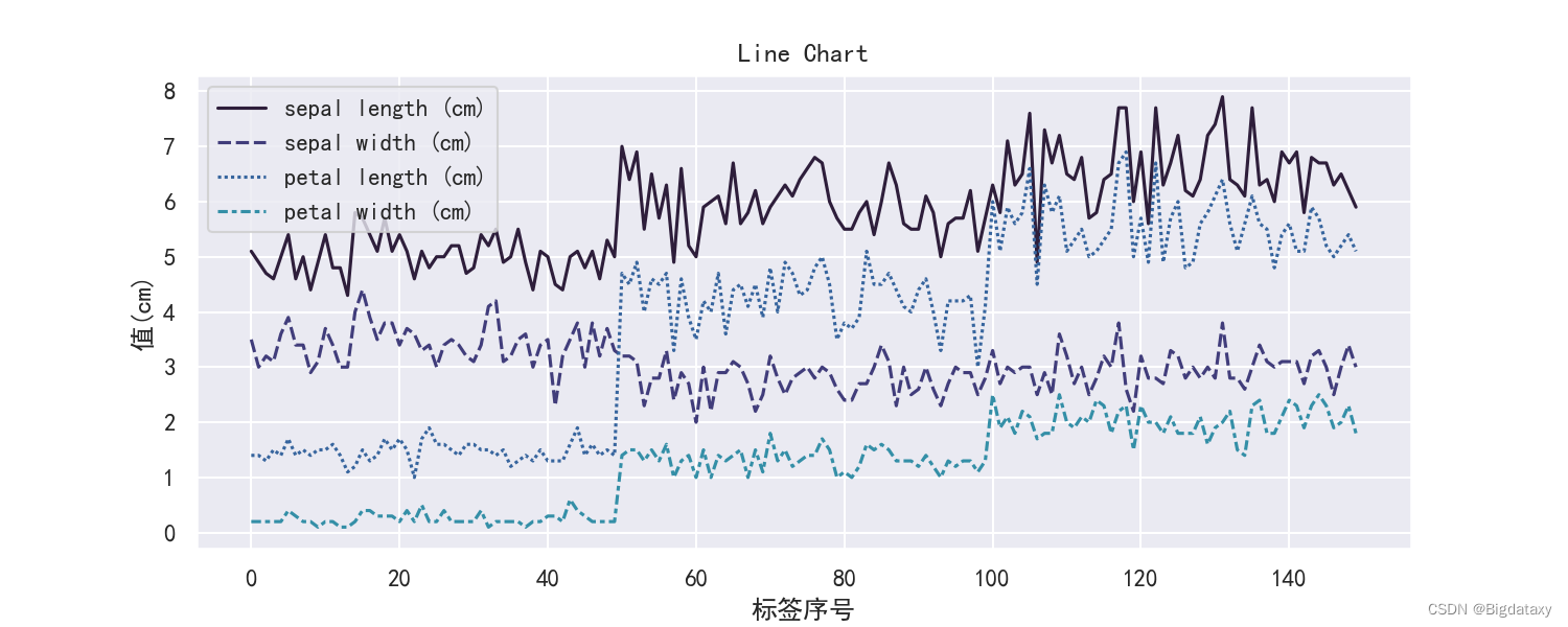
该博客可视化均以iris数据集为基础,现导入需要的包及数据集。 import pandas as pd pd.plotting.register_matplotlib_converters() import matplotlib.pyplot as plt import seaborn as sns from sklearn.datasets import load_iris其中,第二行代码是为了消除matplotlib与seaborn的冲突警告,详细说明可查看我的博客pd.plotting.register_matplotlib_converters() 的作用。 2.读入数据将bunch结构的iris数据集导入,并转换为DataFrame结构方便之后操作。 def bunch2datafram(load_bunchdata): df_data = pd.DataFrame(data = load_bunchdata().data,columns = load_bunchdata().feature_names) df_data['target'] = load_bunchdata().target return df_data df_data = bunch2datafram(load_iris)详细的转换讲解可参考博客Bunch转化为DataFrame的一般方法 3.设置样式该步骤设置一款自己喜欢的调试板,作为后期作图的基础样式,这里运用的是“mako”,个人觉得还不错,喜欢其他的可去官网找找。 sns.set_theme(palette='mako') # 设置样式 plt.rcParams['font.sans-serif']=['SimHei'] # 设置适应模式的字体 plt.rcParams['axes.unicode_minus']=False # 解决坐标负数无法显示的问题这一步也可以不进行,默认的调色板也不错。 三、绘图操作 1.线性图 # Line Charts plt.figure(figsize=(10,4),dpi=150) # figsize设置长宽比,dpi设置像素 sns.lineplot(data=df_data.iloc[:,0:4]) plt.xlabel("标签序号") plt.ylabel("值(cm)") plt.title("Line Chart") ## 下列代码没有实际意义,仅拓展操作思路 # sns.lineplot(data=df_data.iloc[:,0], label=df_data.columns[0]) # sns.lineplot(x=df_data.iloc[:,0],y = df_data.iloc[:,1],hue=df_data["target"])示图样例:
条形图可观察各属性的平均值,代码如下: # Bar Charts plt.figure(figsize=(10,5),dpi=130) sns.barplot(data=df_data.iloc[:,0:4],width=0.4) plt.ylabel("value") plt.title("Bar Chart各属性的平均值")示图样例: 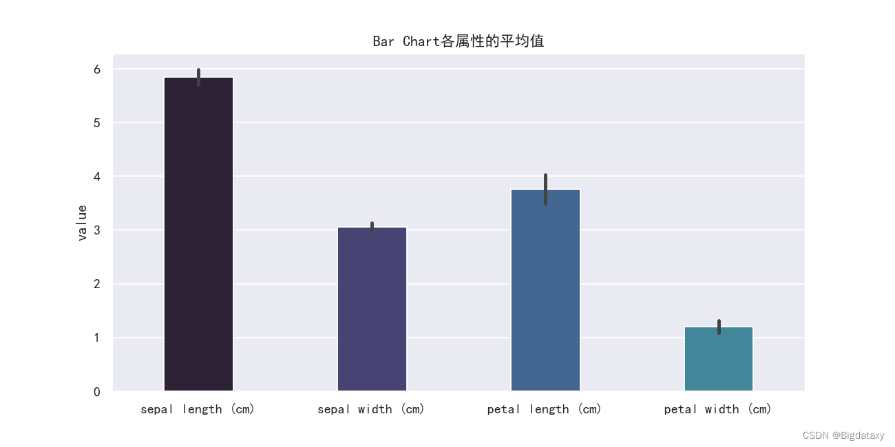
热力图可直观的反映各数据大小,代码如下: # heatmaps plt.figure(figsize=(10,5),dpi=130) sns.heatmap(data=df_data.iloc[40:50,0:4],annot=True) # annot:取True显示值; # 添加图像说明 plt.ylabel("标签序号") plt.xlabel("属性") plt.title("HeatMap")其中设置annot为True即显示图像各小块上面的数值,示图样例如下: 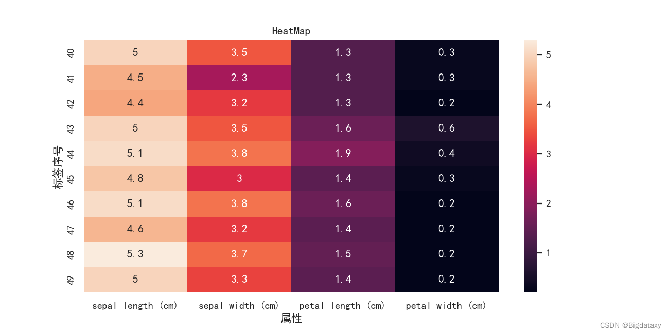 3.散点图
3.散点图
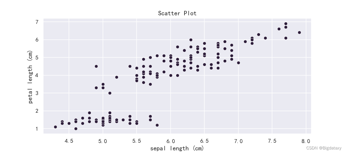
基础散点图,可直观观察不同属性之间的分布关系。 # Scatter Plot plt.figure(figsize=(9,4),dpi=130) sns.scatterplot(x=df_data.iloc[:,0],y= df_data.iloc[:,2]) plt.title("Scatter Plot")示图样例如下: 示图样例如下: 示图样例如下: 示图样例如下: 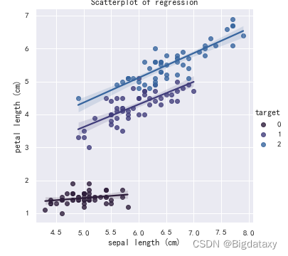
标签箱型散点图,直观呈现各属性值在不同target下的分布情况,同时可作为异常点初步分析的依据。代码如下: plt.figure(figsize=(7,4),dpi=130) sns.swarmplot(x=df_data["target"],y=df_data.iloc[:,0]) plt.title("标签箱型散点图")示图样例如下: 直方图,频数直方图可反映出属性的集中情况与大致分布,其代码如下: plt.figure(figsize=(9,4),dpi=130) sns.histplot(df_data['petal length (cm)']) plt.title("直方图")示图样例如下: 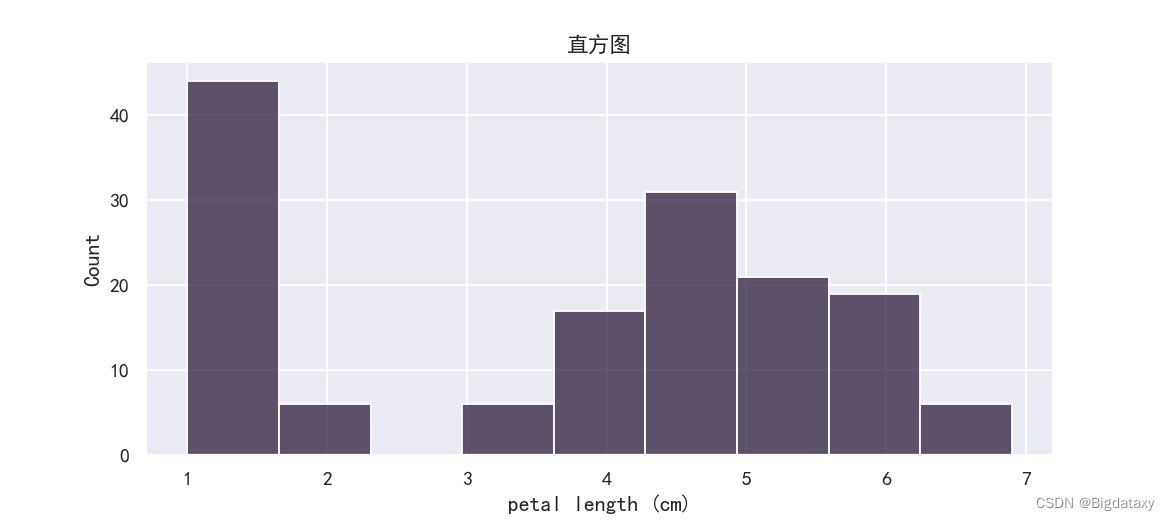
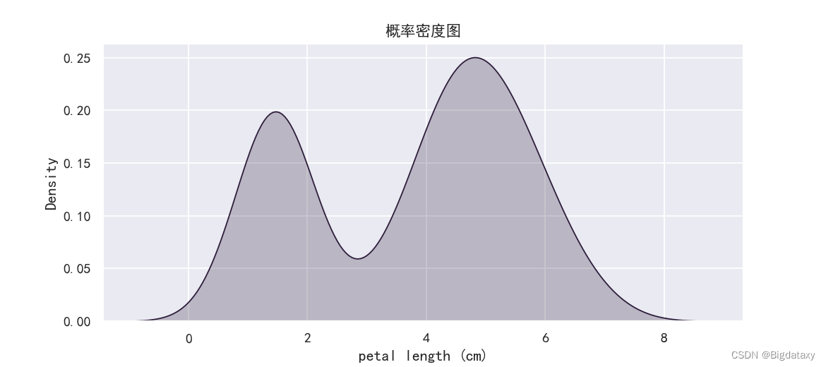
概率密度图(KDE),直观呈现该属性的分布情况,可初步检验是否满足正态分布,代码如下: #KDE plot plt.figure(figsize=(9,4),dpi=130) sns.kdeplot(data=df_data['petal length (cm)'], fill=True) # fill:取True,填充图形下方。 plt.title("概率密度图")示图样例如下: 示图样例如下: 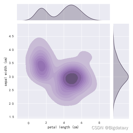
带标签信息的直方图,可直观的观测不同target在该属性下的分布情况,可后面类比特征的提取做准备,代码如下: plt.figure(figsize=(7,4),dpi=130) sns.histplot(data=df_data,x='petal length (cm)',hue = 'target') plt.title("带标签的直方图")示图样例如下: 示图样例如下: 语法:seaborn.pairplot(data, hue=None, hue_order=None, palette=None, vars=None, x_vars=None, y_vars=None, kind=‘scatter’, diag_kind=‘auto’, markers=None, height=2.5, aspect=1, corner=False, dropna=True, plot_kws=None, diag_kws=None, grid_kws=None, size=None) g = sns.pairplot(pd_iris) g.fig.set_size_inches(12,12)#figure大小 sns.set(style='darkgrid',font_scale=1.5)#文本大小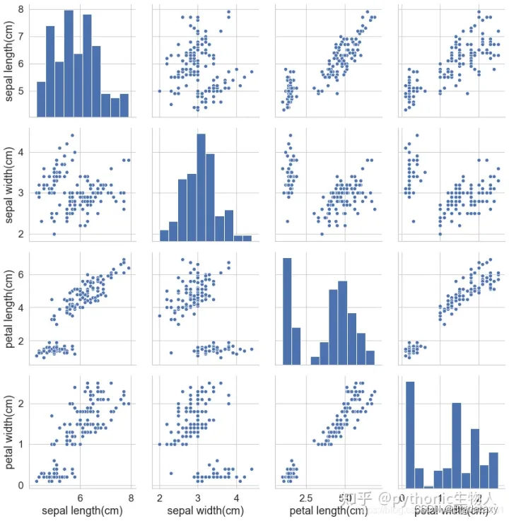
对角线4张图是变量自身的分布直方图; 非对角线的 12 张就是某个变量和另一个变量的关系。 加上分类变量 g = sns.pairplot(pd_iris, hue='class'#按照三种花分类 ) sns.set(style='whitegrid') g.fig.set_size_inches(12,12) sns.set(style='whitegrid',font_scale=1.5)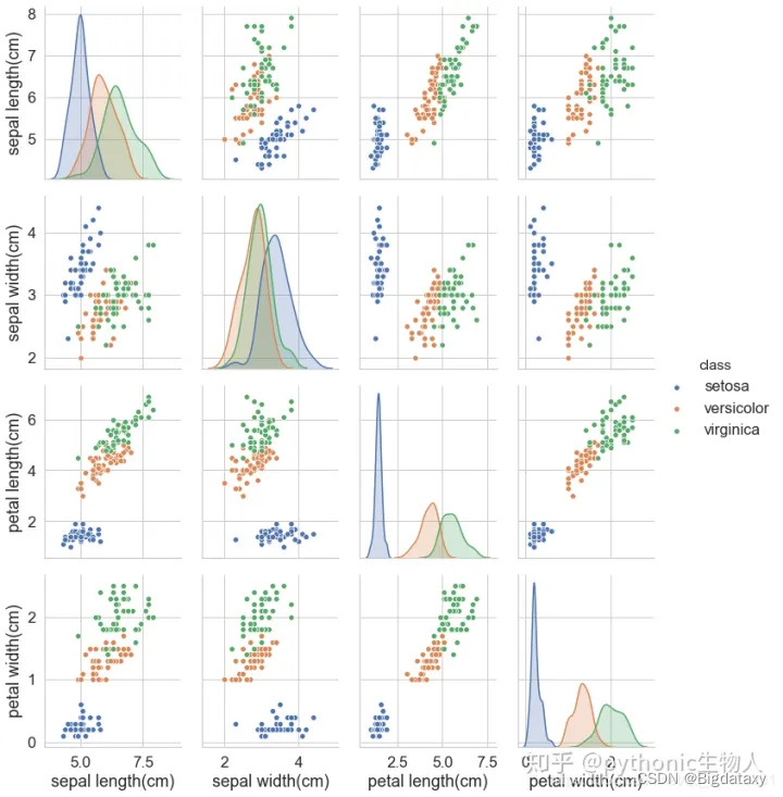 总结
总结
以上就是今天要讲的内容,本文详细的介绍了Seaborn的一般操作,上述记录的方法能较好地满足可视化分析及结果呈现的需求。现对于各种图形的选择,作如下总结: Trends - A trend is defined as a pattern of change. sns.lineplot - Line charts are best to show trends over a period of time, and multiple lines can be used to show trends in more than one group. Relationship - There are many different chart types that you can use to understand relationships between variables in your data. sns.barplot - Bar charts are useful for comparing quantities corresponding to different groups.sns.heatmap - Heatmaps can be used to find color-coded patterns in tables of numbers.sns.scatterplot - Scatter plots show the relationship between two continuous variables; if color-coded, we can also show the relationship with a third categorical variable.sns.regplot - Including a regression line in the scatter plot makes it easier to see any linear relationship between two variables.sns.lmplot - This command is useful for drawing multiple regression lines, if the scatter plot contains multiple, color-coded groups.sns.swarmplot - Categorical scatter plots show the relationship between a continuous variable and a categorical variable. Distribution - We visualize distributions to show the possible values that we can expect to see in a variable, along with how likely they are. sns.histplot - Histograms show the distribution of a single numerical variable.sns.kdeplot - KDE plots (or 2D KDE plots) show an estimated, smooth distribution of a single numerical variable (or two numerical variables).sns.jointplot - This command is useful for simultaneously displaying a 2D KDE plot with the corresponding KDE plots for each individual variable.https://www.kaggle.com/code/alexisbcook/choosing-plot-types-and-custom-styles |
 设置hue值可分别对各target作线性图,示图样例如下:
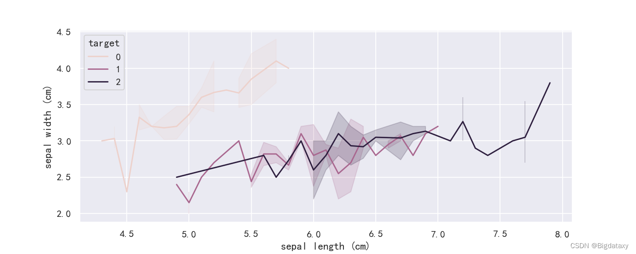
 带有线性回归的散点图,在体现不同属性间分布关系的基础上,做出一条回归直线,可直观观测是否存在线性相关,代码如下:
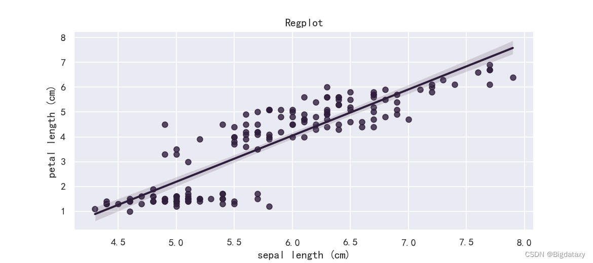 带标签信息的散点图,可直观体现不同属性不同target间的分布关系,代码如下:
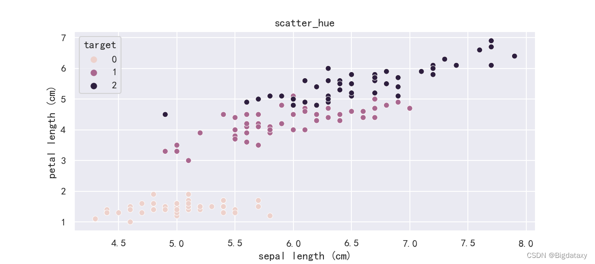 带不同标签回归信息的散点图,可直观观测不同属性在不同标签下,是否呈现线性相关,代码如下:
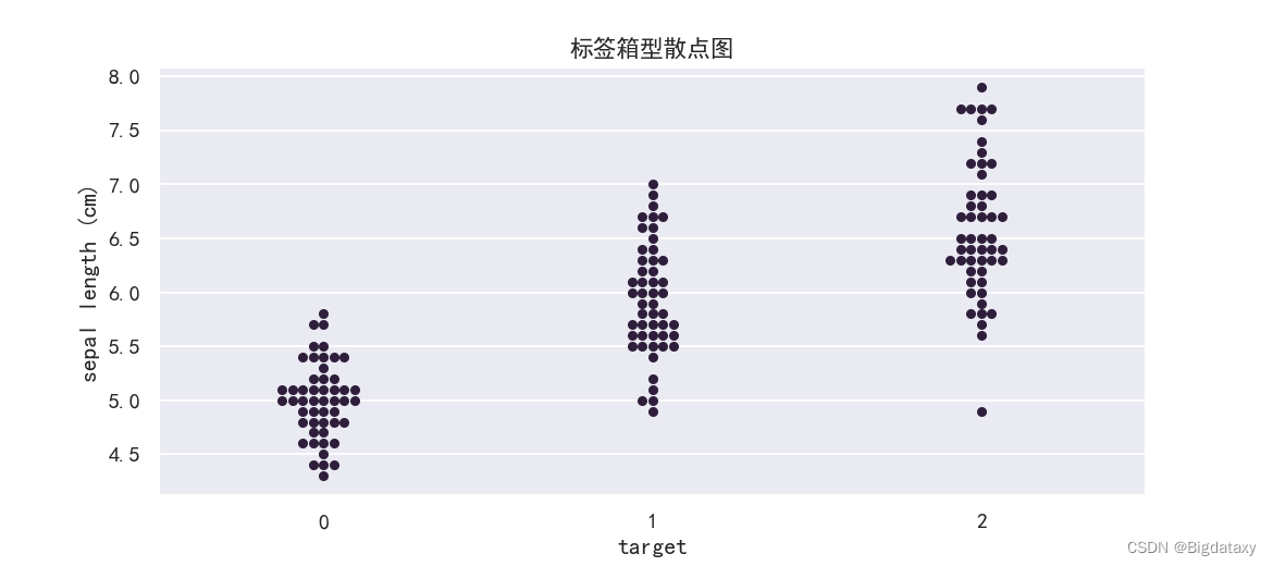
 2维概率密度图(2D KDE),直观呈现两种属性间的整体分布情况,可理解为等高线图,代码如下:
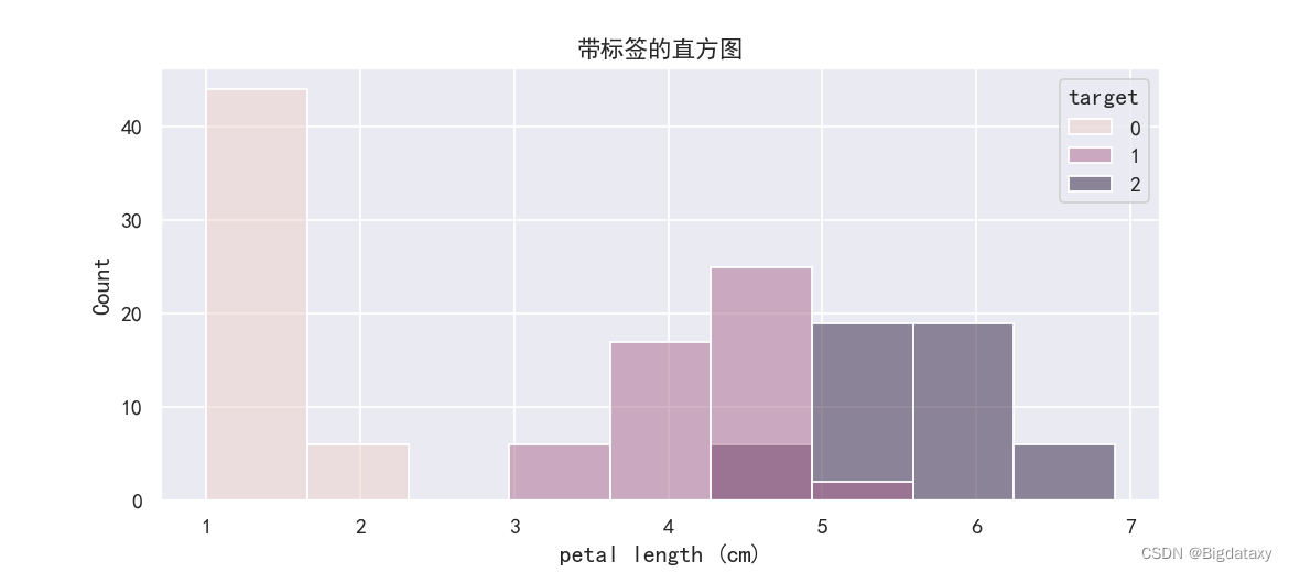 带标签信息的概率密度图,可直观的观测该属性下各target的分布情况,代码如下:
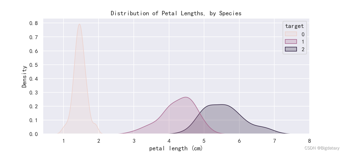
【本文地址】