| 科学网 | 您所在的位置:网站首页 › 截断误差是余项吗 › 科学网 |
科学网
|
截断误差与舍入误差
已有 34277 次阅读 2016-8-15 11:34 |个人分类:数学|系统分类:科研笔记| 差分 (1)在数学中,有限差分方法(Finite Differenc Methods,FDM),是一种微分方程的数值方法,是通过有限差分来近似导数或者偏导数,从而求得微分方法的近似解。在实际中,许多数学问题都很难得到其解析解,所谓解析解就是可以通过给出解的具体函数形式,从解的表达式中就可以算出任何自变量对应值;而数值解是在特定条件下通过近似计算得出来的一个数值。 举个例子: 一般一元二次方程a x^2 + b x + c == 0 (a ≠ 0)的解析解为x = (- b ±√(b^2 - 4 a c)) / (2 a)数值解只能由具体的系数确定。 (2)导数的有限差分近似由泰勒展开的推算 假设f(x)在x0处各阶可导,则根据定理,其在x0+h的泰勒展开式为: {displaystyle f(x_{0}+h)=f(x_{0})+{frac {f'(x_{0})}{1!}}h+{frac {f^{(2)}(x_{0})}{2!}}h^{2}+cdots +{frac {f^{(n)}(x_{0})}{n!}}h^{n}+R_{n}(x),} 其中n!表示是n的階乘,Rn(x)為餘數,表示泰勒多項式和原函數之間的差。可以推導函數f一階導數的近似值: 设定x0=a,可得: {displaystyle f(a+h)=f(a)+f'(a)h+R_{1}(x),} 除以h可得: {displaystyle {f(a+h) over h}={f(a) over h}+f'(a)+{R_{1}(x) over h}} 求解f'(a): {displaystyle f'(a)={f(a+h)-f(a) over h}-{R_{1}(x) over h}} R1(x)是x(x->a时)的高阶无穷小,假设R1(x)很小并可以忽略,可以将"f"的一阶导数近似为: (一阶近似) 定理:设 n 是一个正整数。如果定义在一个包含 a 的区间上的函数 f 在 a 点处 n+1 次可导,那么对于这个区间上的任意 x,都有: {displaystyle f(x)=f(a)+{frac {f'(a)}{1!}}(x-a)+{frac {f^{(2)}(a)}{2!}}(x-a)^{2}+cdots +{frac {f^{(n)}(a)}{n!}}(x-a)^{n}+R_{n}(x).}[2]其中的多项式称为函数在a 处的泰勒展开式,剩余的{displaystyle R_{n}(x)} 是泰勒公式的余项,是{displaystyle (x-a)^{n}} 的高阶无穷小。 由于在近似过程中,我们截断了Rn(x),因此数值差方法本来存在误差,这种由于截断所引起的误差就是结尾误差。 差分的方法有不同分类,如前向,后向和中心差分:
差分还可以分为,explicit and implicit difference 显式方法 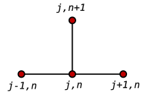 热传导方程最常用显式方法的模版 热传导方程最常用显式方法的模版利用在时间{displaystyle t_{n}}的前向差分,以及在位置{displaystyle x_{j}}的二阶中央差分(FTCS 格式),可以得到以下的迭代方程: {displaystyle {frac {u_{j}^{n+1}-u_{j}^{n}}{k}}={frac {u_{j+1}^{n}-2u_{j}^{n}+u_{j-1}^{n}}{h^{2}}}.,} 这是用求解一维导热传导方程的显式方法。 可以用以下的式子求解{displaystyle u_{j}^{n+1}} {displaystyle u_{j}^{n+1}=(1-2r)u_{j}^{n}+ru_{j-1}^{n}+ru_{j+1}^{n}} 其中{displaystyle r=k/h^{2}.} 因此配合此迭代关系式,已知在时间n的数值,可以求得在时间n+1的数值。{displaystyle u_{0}^{n}}及{displaystyle u_{J}^{n}}的数值可以用边界条件代入,在此例中为0。 此显式方法在{displaystyle rleq 1/2}时,为数值稳定且收敛[1]。其数值误差和时间间隔成正比,和位置间隔的平方成正比: {displaystyle Delta u=O(k)+O(h^{2}),}隐式方法  隐式方法的模版 隐式方法的模版若使用时间{displaystyle t_{n+1}}的后向差分,及位置{displaystyle x_{j}}的二阶中央差分(BTCS 格式),可以得到以下的迭代方程: {displaystyle {frac {u_{j}^{n+1}-u_{j}^{n}}{k}}={frac {u_{j+1}^{n+1}-2u_{j}^{n+1}+u_{j-1}^{n+1}}{h^{2}}}.,} 这是用求解一维导热传导方程的隐式方法。 在求解线性联立方程后可以得到{displaystyle u_{j}^{n+1}}: {displaystyle (1+2r)u_{j}^{n+1}-ru_{j-1}^{n+1}-ru_{j+1}^{n+1}=u_{j}^{n}} 此方法不论{displaystyle r}的大小,都数值稳定且收敛,但在计算量会较显式方法要大,因为每前进一个时间间隔,就需要求解一个联立的数值方程组。其数值误差和时间间隔成正比,和位置间隔的平方成正比: {displaystyle Delta u=O(k)+O(h^{2}),} (3) 舍入误差是由于计算机数字限制(四舍五入)引起的 由于计算机的字长有限,进行数值计算的过程中,对计算得到的中间结果数据要使用“四舍五入”或其他规则取近似值,因而使计算过程有误差。这种误差称为舍入误差。在python中输入0.1+0.2,得到的结果是0.30000000000000004,这是舍入误差带来的结果。 There are two approximations in numerical modelling. One needs to ask the questions: "How well is the natural system modelled by the differential equations?", and, "How well is the solution to the differential equations represented by the computational algorithm?". I n the analysis here more attention is paid to the second question. The first question can only be answered by studying the behaviour of the natural system and comparing i t to the equations applied to it. Therefore i t will be assumed here that the differential equations approximate the system we1 I despite the fact that i t has been noticed that this is not necessarily the case. Abbott (1974) noticed that a difference scheme considerably different from the differential equations used to describe a system, can yield more accurate results than a difference scheme similar to the differential equations when compared with experimental results. There are three possible sources of error associated with finite difference solutions to partial differential equations. I t is important that one understands these sources, their consequence if not control led, and means for controlling them. These three sources of error are: truncation, discretization, and round-off. Truncation error occurs when a derivative is replaced with a finite difference quotient; discretization error is due to the replacement of a continuous model (function) with a discrete model; and round-off error is essentially machine error in that the algebraic finite difference equations are not always solved exactly . For finite difference solutions to be accurate, they must be con- sistent and stable. Consistency simply means that the truncation errors tend to zero as Ax and At - > 0, i.e., as Ax and At - > 0 the finite difference equation becomes the original differential equation. This is examined i n the follcwing paragraphs. Stability implies the controlled growth of round-off error. Stability considerations apply principally to explicit schemes to be discussed later. Any numerical scheme that allows the growth of error, eventually "swamping" the true solution, is unstable. References (1) https://zh.wikipedia.org/zh-cn/%E6%9C%89%E9%99%90%E5%B7%AE%E5%88%86%E6%B3%95 (2) https://zh.wikipedia.org/wiki/%E6%B3%B0%E5%8B%92%E5%85%AC%E5%BC%8F (3) Stephenson, D., kinematic hydrology and modelling. 1986. (4) Chow, E.A., Applied hydrology. 1988. https://blog.sciencenet.cn/blog-922140-996550.html 上一篇:显式与隐式差分下一篇:C语言字符处理 收藏 IP: 210.72.80.*| 热度| |


 (一阶近似)
 [2]
[2] 是泰勒公式的余项,是{displaystyle (x-a)^{n}}
 的高阶无穷小。
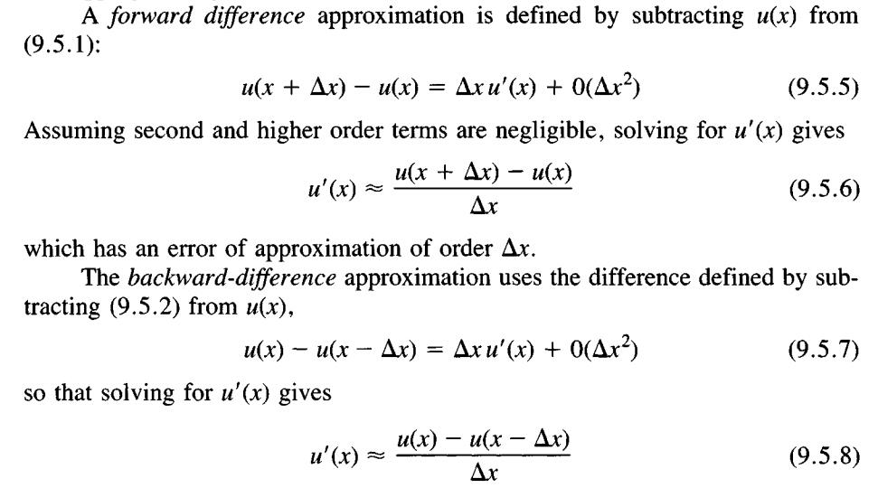
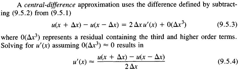 前面两种是对偏微分方程一阶近似,中心差分式二阶近似。
 的前向差分,以及在位置{displaystyle x_{j}}
 的二阶中央差分(FTCS 格式),可以得到以下的迭代方程:


 及{displaystyle u_{J}^{n}}
 的数值可以用边界条件代入,在此例中为0。
 时,为数值稳定且收敛[1]。其数值误差和时间间隔成正比,和位置间隔的平方成正比:
 隐式方法
隐式方法 的后向差分,及位置{displaystyle x_{j}}

 的大小,都数值稳定且收敛,但在计算量会较显式方法要大,因为每前进一个时间间隔,就需要求解一个联立的数值方程组。其数值误差和时间间隔成正比,和位置间隔的平方成正比:
【本文地址】