| 科学网 | 您所在的位置:网站首页 › 态密度分析轨道杂化 › 科学网 |
科学网
|
VASP中杂化泛函优化及态密度计算
已有 19803 次阅读 2014-6-20 12:02 |个人分类:电子结构计算|系统分类:科研笔记 关注:
1) 为避免出错,使计算脚本尽可能简化如分步进行 2) hse的优化及态密度计算 3) GW势 POTCAR_GW能用于杂化泛函计算吗 4) GW或HSE计算时k-mesh如何设置? 在不丧失计算准确性及精度的前提下, 如何提升计算速率?(可以Si为例进行测试)
一、态密度的计算流程思考:
首先是自洽计算(可以是PBE自洽计算、HSE自洽计算或GW自洽计算),这一步比较耗时
其次是“非自洽计算”,利用第一步产生的CHG*文件,设置下列参数进行非自洽计算
ISTART = 1; ICHARG = 11 ISMEAR = -5 LORBIT = 10 # or 11 #Default: ALGO = Normal ;如果第一步自洽计算采用的是HSE或GW自洽,则该处加入:ALGO = None;如第一步是普通的PBE自洽计算,则该处应该加入GW或HSE参数 ## Selects the HSE06 hybrid function #LHFCALC = .TRUE. ; HFSCREEN = 0.2 ; #ALGO = D ; TIME = 0.4
###GW method using POTCAR_GW #ALGO = scGW # ALGO=scGW,GW0,GW,G0W0(if NELM=1) #NELM = 3 # one step so this is really G0W0 #NOMEGA = 50 #if metal, we need a lot of frequency points
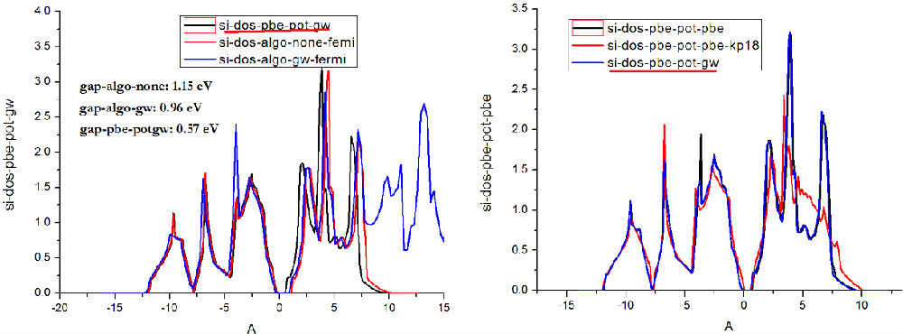
二、Si的态密度测试
结果比较:利用gw计算的WAVECAR、CHG*,(ALGO=none)获得态密度能得到更接近实验值的带隙; gap-algo-gw,为在GW计算的同时,设置LORBIT=11,得到态密度 gap-pbe-potgw:为采用GW赝势,利用PBE方法得到的带隙
Si计算能带(wannier)及DOS(ALGO=none, LORBIT=11)的完整脚本如下:
################## step1: a DFT groundstate calculation ################### cat > INCAR STDOUT cp OUTCAR OUTCAR-01cp STDOUT STDOUT-01 ####################################### step 2: obtain DFT virtual orbitals ##################### cat > INCAR STDOUT cp WAVECAR WAVECAR.LOPTICScp WAVEDER WAVEDER.LOPTICScp OUTCAR OUTCAR-02cp STDOUT STDOUT-02 # #######################step 3: GW + WANNIER90 ################################# cat > INCAR STDOUT cp OUTCAR OUTCAR-03cp STDOUT STDOUTi-03cp WAVECAR WAVECAR-03cp WAVEDER WAVEDER-03
####dos-analysis cat > INCAR STDOUT cp OUTCAR OUTCAR-04cp STDOUT STDOUT-04cp vasprun.xml si-dos-algonone.xml
或
三、Si能带结构测试 可先完成GW计算,利用产生的CHG*,再进行band(LWANNIER90=.TRUE.)计算,也可在GW计算过程中设置LWANNIER90=.TRUE.,得到计算能带所需的wannier90.*文件;两种方法获得的能带时完全重合的: 由此,可见wannier函数真是一种后处理方法?
完整脚本如下:
################## step1: a DFT groundstate calculation ################### cat > INCAR STDOUT cp OUTCAR OUTCAR-01cp STDOUT STDOUT-01 ####################################### step 2: obtain DFT virtual orbitals ##################### cat > INCAR STDOUT cp WAVECAR WAVECAR.LOPTICScp WAVEDER WAVEDER.LOPTICScp OUTCAR OUTCAR-02cp STDOUT STDOUT-02 # #######################step 3: GW -only ################################# cat > INCAR STDOUT cp OUTCAR OUTCAR-03cp STDOUT STDOUTi-03cp WAVECAR WAVECAR-03cp WAVEDER WAVEDER-03 ####band-analysis cat > INCAR STDOUT cp OUTCAR OUTCAR-04cp STDOUT STDOUT-04cp vasprun.xml si-band-algonone.xml 或取消第三步的 #LWANNIER90=.TRUE. 注释,在GW过程中得到能带计算所需的wannier90.*文件
(2)PBE方法计算能带结构的脚本
################## step1: a DFT groundstate calculation ################### cat > INCAR STDOUT cp OUTCAR OUTCAR-01cp STDOUT STDOUT-01 ####step 2: band-analysis cat > INCAR STDOUT cp OUTCAR OUTCAR-02cp STDOUT STDOUT-02cp vasprun.xml si-band-pbe.xml
共用的wannier90.win内容如下:
#num_wann = 64 ! set to NBANDS by VASPnum_wann=8 num_bands=8 # for GW uncomment exclude_bands 9-64 Begin Projections Si:sp3 End Projections dis_froz_max=9 dis_num_iter=1000 guiding_centres=true #use_bloch_phases = T ### Bandstructure plot# restart = plot# bands_plot = true # begin kpoint_path# L 0.50000 0.50000 0.5000 G 0.00000 0.00000 0.0000# G 0.00000 0.00000 0.0000 X 0.50000 0.00000 0.5000# X 0.50000 0.00000 0.5000 K 0.37500 -0.37500 0.0000# K 0.37500 -0.37500 0.0000 G 0.00000 0.00000 0.0000# end kpoint_path # bands_num_points 40# bands_plot_format gnuplot xmgrace
四、 对HSE情形,还能只用wannier函数做后处理吗? 在HSE计算同时设置(LORBIT=11)进行态密度计算,或设置LWANNIER90=.TRUE.进行带结构计算:这样为得到DOS和band需进行两次耗时的HSE计算?!
1.手册实例: http://cms.mpi.univie.ac.at/wiki/index.php/FccNi_DOS
## Plot the spin-polarized DOS of fcc Ni ## at HSE and PBE0 level, and compare with## standard PBE## Better preconverge with PBE first! ################## step1: a DFT groundstate calculation ################### cat > INCAR STDOUT cp OUTCAR OUTCAR-01cp STDOUT STDOUT-01cp vasprun.xml ni-pbe.xml ####################################### step 2: ##################### cat > INCAR STDOUT cp OUTCAR OUTCAR-02cp STDOUT STDOUT-02cp vasprun.xml ni-hse.xml
实例2
http://cms.mpi.univie.ac.at/wiki/index.php/MgO_optimum_mixing
find optimum HSE mixing parameter for MgO
参数释疑:
## HSELHFCALC = .TRUE. ; HFSCREEN = 0.2 ; AEXX = 0.25ALGO = D ; TIME = 0.4 ; LDIAG = .TRUE. ##VASP2WANNIERLWANNIER90=.TRUE.
1. LHFCALC-tag LHFCALC= .TRUE. | .FALSE. Default: LHFCALC=.FALSE. The flag specifies, whether Hartree-Fock type calculations are performed. At the moment, it is recommended to select an all bands simultaneous algorithm, i.e. ALGO=Damped (IALGO=53) or ALGO=All (IALGO=58) in the INCAR file (see Sec. 6.46 6.47). The blocked Davidson algorithm ALGO=Normal is generally rather slow, and in many cases the Pulay mixer will be unable to determine the proper ground-state. We hence recommend to select the blocked Davidson algorithm only in combination with straight mixing or a Kerker like mixing. The following combination have been successfully applied for small and medium sized systems LHFCALC = .TRUE. ; ALGO = Normal ; IMIX = 1 ; AMIX = a Decrease the parameter a until convergence is reached. In most cases, however, it is recommended to use the damped algorithm with suitably chosen timestep. The following setup for the electronic optimization works reliably in most cases: LHFCALC = .TRUE. ; ALGO = Damped ; TIME = 0.4
If convergence is not obtained, it is recommended to reduce the timestep TIME.
2. Amount of exact/DFT exchange and correlation: AEXX, AGGAX, AGGAC and ALDAC tags
AEXX = [real] (fraction of exact exchange) ALDAC= [real] (fraction of LDA correlation energy) AGGAX= [real] (fraction of gradient correction to exchange) AGGAC= [real] (fraction of gradient correction to correlation) Default: AEXX =0.25 for LHFCALC=.TRUE. =0.0 for LHFCALC=.FALSE. Specifies the amount of exact exchange and various other exchange and correlation settings. The sum of the fraction of the exact exchange and LDA exchange is always 1.0, and it is not possible to set the amount of LDA exchange independently. Examples: if AEXX=0.25, 1/4 of the exact exchange is used, and 3/4 of the LDA exchange is added. For AEXX=0.5, half of the exact exchange is used, and one half of the LDA exchange is added.
The GGA flags AGGAX and AGGAC are only used if GGA is already selected (for LDA type calculations no gradient correction will be added regardless of the values supplied for AGGAX and AGGAC).
Note: The defaults are chosen such that the hybrid PBE0 functional is selected for PBE pseudopotentials (the PBE0 functional contains 25 % of the exact exchange, and 75 % of the PBE exchange, and 100 % of the PBE correlation energy). The resulting expression for the exchange-correlation energy then takes the following simple form:
 (6.64) (6.64)
Other sensible values are of course AEXX=1.0 (full Hartree-Fock type calculations). In this case, VASP also automatically selects ALDAC=0.0 and AGGAC=0.0, to avoid the addition of a (semi-local) correlation energy. A comprehensive evaluation of the performance of the PBE0 functional, as compared to PBE, can be found in Ref. [92].
3. IALGO, and LDIAG-tag IALGO = 38 | 48 LDIAG = .TRUE. | .FALSE. Default IALGO = 8 for VASP.4.4 and older = 38 for VASP.4.5, VASP.4.6 and VASP.5.2 (if ALGO is not set) LDIAG = .TRUE. IALGO = integer selecting algorithm LDIAG = perform sub space rotation Please mind, that the VASP.4.5 default is IALGO = 38 (a Davidson block iteration scheme). IALGO = 8 is not supported for copyright reasons in VASP.4.5, but IALGO = 38 is roughly 2 times faster for large systems than IALGO = 8 and at least as stable. You can select the algorithm also by setting ALGO= Normal | Fast | Very_Fast in the INCAR file (see Sec. 6.46). IALGO selects the main algorithm, and LDIAG determines whether a subspace-diagonalization is performed, or not. We strongly urge the users to set the algorithms via ALGO. Algorithms other than those available via ALGO are subject to instabilities. Generally the first digit of IALGO specifies the main algorithm, the second digit controls the actual settings within the algorithm. For instance 4X will always call the same routine for the electronic minimization the second digit X controls the details of the electronic minimization (preconditioning etc.).
For small gap systems and for metals, it is however usually required (metals) or desirable (semiconductors) to use a larger value for NBANDS. In this case, we recommend to use the damped MD algorithm (IALGO = 53, ALGO = Damped) instead of the conjugate gradient one. The stability of the all bands simultaneously algorithms depends strongly on the setting of TIME. For the conjugate gradient case, TIME controls the step size in the trial step, which is required in order to perform a line minimization of the energy along the gradient (or conjugated gradient, see section 6.22 for details). Too small steps make the line minimization less accurate, whereas too large steps can cause instabilities. The step size is usually automatically scaled by the actual step size minimizing the total energy along the gradient (values can range from 1.0 for insulators to 0.01 for metals with a large density of states at the Fermi-level).
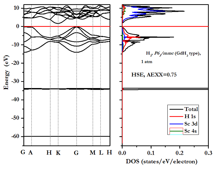
XH3计算的成功脚本-HSE-DOS计算:
态密度少了60电子伏附近的,为何?
################## step 1: a DFT groundstate calculation , and get DOS and band ################### cat > INCAR STDOUT cp OUTCAR OUTCAR-01cp STDOUT STDOUT-01
#######################step 2: Doing the HSE hybrid functional for comparison ################################# cat > INCAR STDOUT cp OUTCAR OUTCAR-02cp STDOUT STDOUT-02
https://blog.sciencenet.cn/blog-567091-805015.html 上一篇:VASP中的杂化泛函计算方法下一篇:LSDA+U计算VASP算例分析 收藏 IP: 139.205.190.*| 热度| |

【本文地址】
| 今日新闻 |
| 推荐新闻 |
| 专题文章 |