异常检测算法：孤立森林（isolation forest）的python代码实现

#异常检测算法：孤立森林（isolation forest）的python代码实现| 来源: 网络整理| 查看: 265

文章目录孤立森林算法简介代码实现可视化

孤立森林算法简介

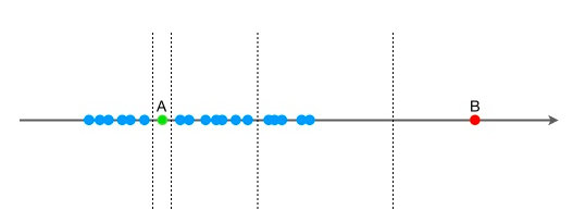
孤立森林是一种无监督学习算法，可以用来做anomaly detection。在孤立森林中，递归地随机分割数据集，直到所有的样本点都是孤立的。在这种随机分割的策略下，通常只需要极少的分割次数就可以使得异常点被孤立。换句话说，那些密度很高的簇是需要被切割很多次才能被孤立，但是那些密度很低的点很容易就可以被孤立。

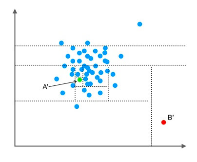
将一维空间拓展到二维空间也是如此，异常点可以很快地被切割成孤立点。

代码实现

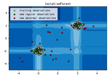
使用sklearn中的相关包来实现孤立森林算法，举一个很简单的小demo：

from sklearn.ensemble import IsolationForest X = [[-1.1], [0.2], [10.1], [0.3], [2.5], [1.7], [2.2], [1.7]] clf = IsolationForest() clf.fit(X) # 输出decision_function的结果：大于0表示正样本的可信度大于负样本，否则可信度小于负样本。 # 在这个demo中，第三个数字是异常点的可能性最大，其次是第一个数字 scores = clf.decision_function(X) """ 输出的结果是： [-0.10780172 0.08482445 -0.2449808 0.08846511 0.04413297 0.11703052 0.0870313 0.11703052] """ print(scores)

其他的内置函数以及介绍在：scikit-learn

可视化

sklearn上的可视化案例，链接为scikit-learn-iForest-demo

import numpy as np import matplotlib.pyplot as plt from sklearn.ensemble import IsolationForest rng = np.random.RandomState(42) # Generate train data X = 0.3 * rng.randn(100, 2) X_train = np.r_[X + 2, X - 2] # Generate some regular novel observations X = 0.3 * rng.randn(20, 2) X_test = np.r_[X + 2, X - 2] # Generate some abnormal novel observations X_outliers = rng.uniform(low=-4, high=4, size=(20, 2)) # fit the model clf = IsolationForest(max_samples=100, random_state=rng) clf.fit(X_train) y_pred_train = clf.predict(X_train) y_pred_test = clf.predict(X_test) y_pred_outliers = clf.predict(X_outliers) # plot the line, the samples, and the nearest vectors to the plane xx, yy = np.meshgrid(np.linspace(-5, 5, 50), np.linspace(-5, 5, 50)) Z = clf.decision_function(np.c_[xx.ravel(), yy.ravel()]) Z = Z.reshape(xx.shape) plt.title("IsolationForest") plt.contourf(xx, yy, Z, cmap=plt.cm.Blues_r) b1 = plt.scatter(X_train[:, 0], X_train[:, 1], c='white', s=20, edgecolor='k') b2 = plt.scatter(X_test[:, 0], X_test[:, 1], c='green', s=20, edgecolor='k') c = plt.scatter(X_outliers[:, 0], X_outliers[:, 1], c='red', s=20, edgecolor='k') plt.axis('tight') plt.xlim((-5, 5)) plt.ylim((-5, 5)) plt.legend([b1, b2, c], ["training observations", "new regular observations", "new abnormal observations"], loc="upper left") plt.show()

最终的结果是：

其中，红色即为异常点，白色是训练集，绿色是测试数据。

【本文地址】

公司简介

联系我们

今日新闻

推荐新闻

专题文章