| 使用奇异值分解(SVD)压缩图片(python实现) | 您所在的位置:网站首页 › 奇异值分解求法 › 使用奇异值分解(SVD)压缩图片(python实现) |
使用奇异值分解(SVD)压缩图片(python实现)
|
奇异值分解压缩图片原理
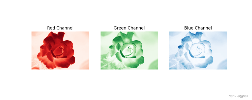
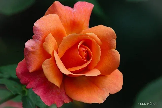
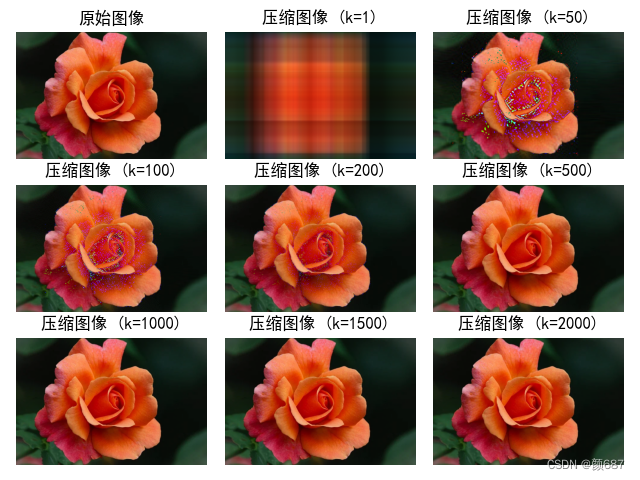
图片在计算机内以矩阵形式存储,因此可以使用矩阵论知识和算法对数字图像(图片)进行分析与处理。 原理简述彩色图片有3个图层,分别显示3个通道(红、绿、蓝),彩色图片就是3个图层混合才能表示不同的色彩。对3个图层分别进行奇异值分解,可以选取前k个奇异值进行近似表达(每个矩阵的奇异值是唯一的,矩阵大小跟奇异值数量有关),最后合并3个图层就可以以较少的数据表示原图片(也就是使用多于原图片奇异值数量的奇异值可能会使图片更大)。
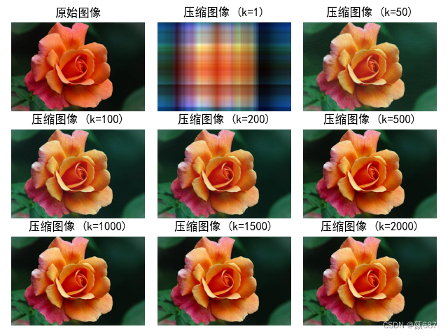
可以看到不同的奇异值对图片的压缩有不同的效果,分辨率越低的图片的奇异值数量越低,过高的奇异值会使图片的大小更大。 上面的代码显示的图片就是SVD对图片压缩的影响,我们可以看到低奇异值压缩得到的图片会有一些花斑,这些花斑是因为图片的像素亮度差较大造成的,如果我们对图像像素的亮度进行归一化,我们就会得到不错的显示效果。下面是加入归一化的代码。 import numpy as np from PIL import Image import matplotlib.pyplot as plt import os # 加载原始彩色图像 original_image = Image.open("flower.jpg") # 将图像转换为NumPy数组 image_array = np.array(original_image) print(f"原图像文件大小{image_array.size} bits\n") # 对每个颜色通道分别进行SVD压缩 def compress_svd(image, k): U, S, V = np.linalg.svd(image, full_matrices=False) #分解原图像 #对原图像的矩阵进行压缩 compressed_U = U[:, :k] compressed_S = np.diag(S[:k]) compressed_V = V[:k, :] compressed_image = np.dot(compressed_U, np.dot(compressed_S, compressed_V)) #对矩阵进行乘法运算,恢复压缩图像 normalized_image = normalize_image(compressed_image) # 对压缩后的图像进行归一化,使用归一化的图像在亮度上会比较均衡,显示效果好 return normalized_image, compressed_U.size, compressed_S.size, compressed_V.size #对压缩后的图像进行归一化 def normalize_image(image): # 将图像矩阵的像素值缩放到0到255的范围内 min_pixel = np.min(image) max_pixel = np.max(image) normalized_image = 255 * (image - min_pixel) / (max_pixel - min_pixel) # 将浮点数像素值转换为无符号整数(uint8) normalized_image = normalized_image.astype(np.uint8) return normalized_image # 设置奇异值列表(不同的压缩级别) singular_values_list = [1, 50, 100, 200, 500, 1000, 1500, 2000] #奇异值大小跟图像大小(分辨率)有关,越大的分辨率可以使用更大的奇异值 # 初始化一个列表以存储压缩后的图像 compressed_images = [] # 对每个奇异值进行压缩 for k in singular_values_list: compressed_image = np.empty_like(image_array, dtype=np.uint8) #创建一个形状与原图形同的空矩阵,用于存放压缩后的矩阵乘积 for channel in range(3): compressed_channel, U_size, S_size, V_size = compress_svd(image_array[:, :, channel], k) compressed_image[:, :, channel] = compressed_channel compressed_images.append(compressed_image) # 将压缩图像转换为Pillow图像对象并保存 for k, compressed_image in zip(singular_values_list, compressed_images): compressed_image = Image.fromarray(compressed_image) compressed_image.save(f"compressed_image_{k}.jpg") # 计算并打印原图像和压缩图像的文件大小 original_file_size = os.path.getsize("original_image.jpg") * 8 #根据图像像素空间大小计算压缩率 compressed_file_sizes = [os.path.getsize(f"compressed_image_{k}.jpg") * 8 for k in singular_values_list] #计算图片压缩率 for k, compressed_size in zip(singular_values_list, compressed_file_sizes): rate = round((original_file_size - compressed_size) / original_file_size, 4) * 100 compressed_image, U_size, S_size, V_size = compress_svd(image_array[:, :, channel], k) #图像传输过程中不是直接传输图像,而是传输图像的矩阵,SVD对图像矩阵进行拆分 transmit_rate = round((image_array.size - 3 * (U_size + S_size + V_size))/image_array.size, 4) * 100 print(f"压缩图像 (k={k}) 文件大小: {compressed_size} bits") print(f"图像大小压缩率 (k={k}): {rate}%") print(f"传输压缩率(k={k}):{transmit_rate}%") # 显示原始图像和8个不同压缩级别的图像 plt.rcParams["font.sans-serif"] = "SimHei" # 解决中文显示问题 plt.figure()#自适应 # plt.figure(figsize=(10, 8)) # 显示原始图像 plt.subplot(3, 3, 1) plt.title("原始图像") plt.imshow(original_image) plt.axis("off") # 显示压缩图像 for i, (k, compressed_image) in enumerate(zip(singular_values_list, compressed_images)): plt.subplot(3, 3, i + 2) plt.title(f"压缩图像 (k={k})") plt.imshow(compressed_image) plt.axis("off") plt.tight_layout() plt.show()
进行归一化的图片显示效果更好,但是因为图片亮度趋于中值,因此也会使图片显示效果不像原图。亮的地方变暗,暗的地方变亮。 对SVD的讲解参考了下面的文章: 基于奇异值分解(SVD)的图片压缩实践 |
【本文地址】
公司简介
联系我们