| 无监督学习 | 您所在的位置:网站首页 › 多维特征聚类分析方法 › 无监督学习 |
无监督学习
|
文章目录
1. KMeans in Sklearn2. Sklearn 实例:电影评分的 k 均值聚类2.1 数据集概述2.2 二维 KMeans 聚类
3. 肘部法选取最优 K 值4. 多维 KMeans 聚类4.1 三维 KMeans 聚类4.2 高维 KMeans 聚类4.2.1 热力图可视化4.2.2 稀疏 csr 矩阵4.2.3 利用聚类结果进行预测4.2.4 利用聚类结果进行推荐
相关文章:
机器学习 | 目录 机器学习 | 聚类评估指标 机器学习 | 距离计算 无监督学习 | KMeans与KMeans++原理 关于 KMeans 以及 KMeans++ 算法原理以及参数的意义,可以参考这篇文章:无监督学习 | KMeans与KMeans++原理 本文将着重讲 KMeans 算法的实现、 K 值的选取以及聚类结果可视化。 1. KMeans in Sklearnsklearn.cluster.KMeans KMeans(n_clusters=8, init='k-means++', n_init=10, max_iter=300, tol=0.0001, precompute_distances='auto', verbose=0, random_state=None, copy_x=True, n_jobs=None, algorithm='auto')参数设置: n_clusters: int, optional, default: 8 The number of clusters to form as well as the number of centroids to generate. 【簇个数】init: {‘k-means++’, ‘random’ or an ndarray} Method for initialization, defaults to ‘k-means++’: ‘k-means++’ : selects initial cluster centers for k-mean clustering in a smart way to speed up convergence. See section Notes in k_init for more details. 【KMeans++,选取一个随机初始向量并通过轮盘法选取剩余k-1个初始向量】 ‘random’: choose k observations (rows) at random from data for the initial centroids. 【传统KMeans,随机选取k个初始向量】 If an ndarray is passed, it should be of shape (n_clusters, n_features) and gives the initial centers.n_init: int, default: 10 Number of time the k-means algorithm will be run with different centroid seeds. The final results will be the best output of n_init consecutive runs in terms of inertia. 【通过多次生成初始点,选取最好的结果】max_iter: int, default: 300 Maximum number of iterations of the k-means algorithm for a single run.【最大的迭代次数】tol: float, default: 1e-4 Relative tolerance with regards to inertia to declare convergence 【最小调整幅度阈值】precompute_distances: {‘auto’, True, False} Precompute distances (faster but takes more memory). ‘auto’ : do not precompute distances if n_samples * n_clusters > 12 million. This corresponds to about 100MB overhead per job using double precision. True : always precompute distances False : never precompute distancesverbose: int, default 0 Verbosity mode.random_state: int, RandomState instance or None (default) Determines random number generation for centroid initialization. Use an int to make the randomness deterministic. See Glossary.copy_x: boolean, optional When pre-computing distances it is more numerically accurate to center the data first. If copy_x is True (default), then the original data is not modified, ensuring X is C-contiguous. If False, the original data is modified, and put back before the function returns, but small numerical differences may be introduced by subtracting and then adding the data mean, in this case it will also not ensure that data is C-contiguous which may cause a significant slowdown.n_jobs: int or None, optional (default=None) The number of jobs to use for the computation. This works by computing each of the n_init runs in parallel. None means 1 unless in a joblib.parallel_backend context. -1 means using all processors. See Glossary for more details. 【多线程】algorithm: “auto”, “full” or “elkan”, default=”auto” K-means algorithm to use. The classical EM-style algorithm is “full”. The “elkan” variation is more efficient by using the triangle inequality, but currently doesn’t support sparse data. “auto” chooses “elkan” for dense data and “full” for sparse data.Attributes: cluster_centers_: array, [n_clusters, n_features] Coordinates of cluster centers. If the algorithm stops before fully converging (see tol and max_iter), these will not be consistent with labels_.labels_: array, shape (n_samples,) Labels of each pointinertia_: float Sum of squared distances of samples to their closest cluster center.n_iter_: int Number of iterations run. 2. Sklearn 实例:电影评分的 k 均值聚类我们将使用的数据来自 MovieLens 用户评分数据集,根据用户对不同电影的评分研究用户在电影品位上的相似和不同之处。 2.1 数据集概述该数据集有两个文件。我们将这两个文件导入 pandas dataframe 中: import pandas as pd import matplotlib.pyplot as plt import numpy as np from scipy.sparse import csr_matrix # Import the Movies dataset movies = pd.read_csv('k-means_Clustering of Movie Ratings/ml-latest-small/movies.csv') movies.head() movieIdtitlegenres01Toy Story (1995)Adventure|Animation|Children|Comedy|Fantasy12Jumanji (1995)Adventure|Children|Fantasy23Grumpier Old Men (1995)Comedy|Romance34Waiting to Exhale (1995)Comedy|Drama|Romance45Father of the Bride Part II (1995)Comedy # Import the ratings dataset ratings = pd.read_csv('k-means_Clustering of Movie Ratings/ml-latest-small/ratings.csv') ratings.head() userIdmovieIdratingtimestamp01312.512607591441110293.012607591792110613.012607591823111292.012607591854111724.01260759205 print('The dataset contains: ', len(ratings), ' ratings of ', len(movies), ' movies.') The dataset contains: 100004 ratings of 9125 movies.现在我们已经知道数据集的结构,可以看到总共有 100004 条影评,对应于 9125 部影片。 电影的类型大致有:喜剧、浪漫、儿童、漫画… 2.2 二维 KMeans 聚类我们想要看看在观众中,对于爱情片和科幻片的评分是否有明显的分类,我们通过计算每位用户对爱情片和科幻片的评分,并对数据集稍微进行偏倚(删除同时喜欢科幻片和爱情片的用户),使聚类能够将他们定义为更喜欢其中一种类型。 我们将大部分数据预处理过程都隐藏在了辅助函数 helper 中,并重点研究聚类概念。 import helper # Calculate the average rating of romance and scifi movies genre_ratings = helper.get_genre_ratings(ratings, movies, ['Romance', 'Sci-Fi'], ['avg_romance_rating', 'avg_scifi_rating']) # 函数 get_genre_ratings 计算了每位用户对所有爱情片和科幻片的平均评分。我们对数据集稍微进行偏倚,删除同时喜欢科幻片和爱情片的用户,使聚类能够将他们定义为更喜欢其中一种类型。 biased_dataset = helper.bias_genre_rating_dataset(genre_ratings, 3.2, 2.5) print( "Number of records: ", len(biased_dataset)) biased_dataset.head() Number of records: 183 indexavg_romance_ratingavg_scifi_rating013.502.40133.653.14262.902.75372.933.364122.892.62可以看出我们有 183 位用户,对于每位用户,我们都得出了他们对看过的爱情片和科幻片的平均评分。 我们来绘制该数据集: %matplotlib inline helper.draw_scatterplot(biased_dataset['avg_scifi_rating'],'Avg scifi rating', biased_dataset['avg_romance_rating'], 'Avg romance rating')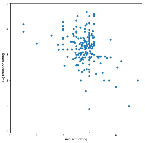
我们可以在此样本中看到明显的偏差(我们故意创建的)。如果使用 k 均值将样本分成两组,效果如何? # Let's turn our dataset into a list X = biased_dataset[['avg_scifi_rating','avg_romance_rating']].values from sklearn.cluster import KMeans kmeans_1 = KMeans(n_clusters=2) predictions = kmeans_1.fit_predict(X) # Plot helper.draw_clusters(biased_dataset, predictions)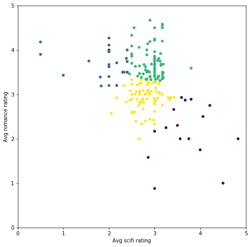
可以看出分组的依据主要是每个人对爱情片的评分高低。如果爱情片的平均评分超过 3 星,则属于第一组,否则属于另一组。 如果分成三组,会发生什么? kmeans_2 = KMeans(n_clusters=3) predictions_2 = kmeans_2.fit_predict(X) # Plot helper.draw_clusters(biased_dataset, predictions_2)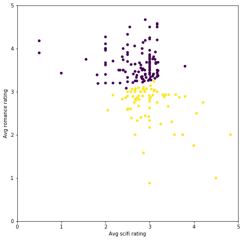
现在平均科幻片评分开始起作用了,分组情况如下所示: 喜欢爱情片但是不喜欢科幻片的用户喜欢科幻片但是不喜欢爱情片的用户即喜欢科幻片又喜欢爱情片的用户再添加一组: kmeans_3 = KMeans(n_clusters=4) predictions_3 = kmeans_3.fit_predict(X) # Plot helper.draw_clusters(biased_dataset, predictions_3)
可以看出将数据集分成的聚类越多,每个聚类中用户的兴趣就相互之间越相似。 3. 肘部法选取最优 K 值我们可以将数据点拆分为任何数量的聚类。对于此数据集来说,正确的聚类数量是多少? 可以通过多种方式选择聚类 k。我们将研究一种简单的方式,叫做“肘部方法”。肘部方法会绘制 k 的上升值与使用该 k 值计算的总误差分布情况。 其思想与网络搜索类似,通过遍历参数 K 来选取最小误差,我们这里选取轮廓系数(约接近 1 性能越好)来评价聚类性能。 现在的一个任务是对每个 k(介于 1 到数据集中的元素数量之间,以 5 为步长)执行相同的操作。 df = biased_dataset[['avg_scifi_rating','avg_romance_rating']] # Choose the range of k values to test. # We added a stride of 5 to improve performance. We don't need to calculate the error for every k value possible_k_values = range(2, len(X)+1, 5) # Calculate error values for all k values we're interested in errors_per_k = [helper.clustering_errors(k, X) for k in possible_k_values] # Plot the each value of K vs. the silhouette score at that value fig, ax = plt.subplots(figsize=(16, 6)) plt.plot(possible_k_values, errors_per_k) # Ticks and grid xticks = np.arange(min(possible_k_values), max(possible_k_values)+1, 5.0) ax.set_xticks(xticks, minor=False) ax.set_xticks(xticks, minor=True) ax.xaxis.grid(True, which='both') yticks = np.arange(round(min(errors_per_k), 2), max(errors_per_k), .05) ax.set_yticks(yticks, minor=False) ax.set_yticks(yticks, minor=True) ax.yaxis.grid(True, which='both')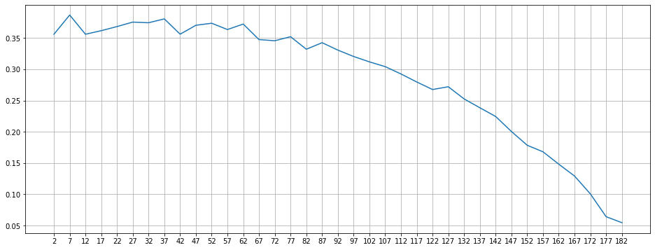
看了该图后发现,合适的 k 值包括 7、22、27、32 等(每次运行时稍微不同)。聚类 (k) 数量超过该范围将开始导致糟糕的聚类情况(根据轮廓分数) 我会选择 k=7,因为更容易可视化: kmeans_4 = KMeans(n_clusters=7) predictions_4 = kmeans_4.fit_predict(X) # Plot helper.draw_clusters(biased_dataset, predictions_4, cmap='Accent')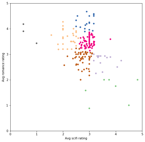
注意:当你尝试绘制更大的 k 值(超过 10)时,需要确保你的绘制库没有对聚类重复使用相同的颜色。对于此图,我们需要使用 matplotlib colormap Accent,因为其他色图要么颜色之间的对比度不强烈,要么在超过 8 个或 10 个聚类后会重复利用某些颜色。 4. 多维 KMeans 聚类 4.1 三维 KMeans 聚类到目前为止,我们只查看了用户如何对爱情片和科幻片进行评分。我们再添加另一种类型,看看加入动作片类型后效果如何。 现在数据集如下所示: biased_dataset_3_genres = helper.get_genre_ratings(ratings, movies, ['Romance', 'Sci-Fi', 'Action'], ['avg_romance_rating', 'avg_scifi_rating', 'avg_action_rating']) biased_dataset_3_genres = helper.bias_genre_rating_dataset(biased_dataset_3_genres, 3.2, 2.5).dropna() print( "Number of records: ", len(biased_dataset_3_genres)) biased_dataset_3_genres.head() Number of records: 183 indexavg_romance_ratingavg_scifi_ratingavg_action_rating013.502.402.80133.653.143.47262.902.753.27372.933.363.294122.892.623.21对三维数据进行聚类并通过三维平面图可视化。 我们依然分别用 x 轴和 y 轴表示科幻片和爱情片。并用点的大小大致表示动作片评分情况(更大的点表示平均评分超过 3 颗星,更小的点表示不超过 3 颗星 )。 X_with_action = biased_dataset_3_genres[['avg_scifi_rating', 'avg_romance_rating', 'avg_action_rating']].values kmeans_5 = KMeans(n_clusters=7) predictions_5 = kmeans_5.fit_predict(X_with_action) # plot helper.draw_clusters_3d(biased_dataset_3_genres, predictions_5)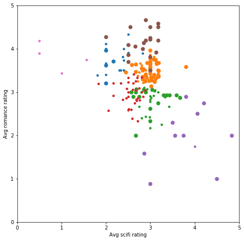
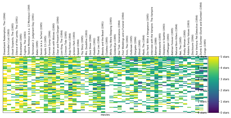
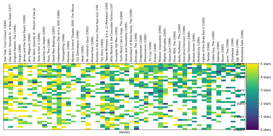
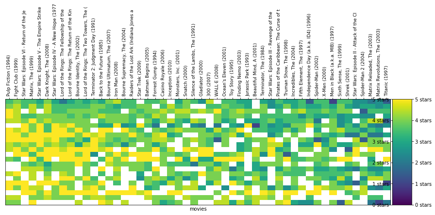
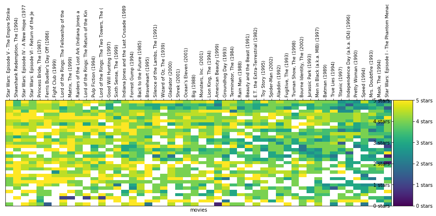
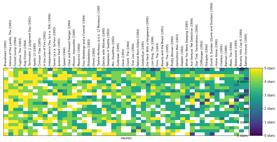
可以看出添加类型后,用户的聚类分布发生了变化。为 k 均值提供的数据越多,每组中用户之间的兴趣越相似。但是如果继续这么绘制,我们将无法可视化二维或三维之外的情形。在下个部分,我们将使用另一种图表,看看多达 50 个维度的聚类情况。 4.2 高维 KMeans 聚类现在我们已经知道 k 均值会如何根据用户的类型品位对用户进行聚类,我们再进一步分析,看看用户对单个影片的评分情况。为此,我们将数据集构建成 userId 与用户对每部电影的评分形式。例如,我们来看看以下数据集子集: # Merge the two tables then pivot so we have Users X Movies dataframe ratings_title = pd.merge(ratings, movies[['movieId', 'title']], on='movieId' ) user_movie_ratings = pd.pivot_table(ratings_title, index='userId', columns= 'title', values='rating') print('dataset dimensions: ', user_movie_ratings.shape, '\n\nSubset example:') user_movie_ratings.iloc[:6, :10] dataset dimensions: (671, 9064) Subset example: title"Great Performances" Cats (1998)$9.99 (2008)'Hellboy': The Seeds of Creation (2004)'Neath the Arizona Skies (1934)'Round Midnight (1986)'Salem's Lot (2004)'Til There Was You (1997)'burbs, The (1989)'night Mother (1986)(500) Days of Summer (2009)userId1NaNNaNNaNNaNNaNNaNNaNNaNNaNNaN2NaNNaNNaNNaNNaNNaNNaNNaNNaNNaN3NaNNaNNaNNaNNaNNaNNaNNaNNaNNaN4NaNNaNNaNNaNNaNNaNNaNNaNNaNNaN5NaNNaNNaNNaNNaNNaNNaNNaNNaNNaN6NaNNaNNaNNaNNaNNaNNaN4.0NaNNaNNaN 值表明了一个问题。大多数用户没有看过大部分电影,并且没有为这些电影评分。这种数据集称为“稀疏”数据集,因为只有少数单元格有值。 为了解决这一问题,我们按照获得评分次数最多的电影和对电影评分次数最多的用户排序。这样可以形成更“密集”的区域,使我们能够查看数据集的顶部数据。 如果我们要选择获得评分次数最多的前 30 部电影和对电影评分次数最多的 18 个用户,则如下所示: n_movies = 30 n_users = 18 most_rated_movies_users_selection = helper.sort_by_rating_density(user_movie_ratings, n_movies, n_users) print('dataset dimensions: ', most_rated_movies_users_selection.shape) most_rated_movies_users_selection.head() dataset dimensions: (18, 30) titleForrest Gump (1994)Pulp Fiction (1994)Shawshank Redemption, The (1994)Silence of the Lambs, The (1991)Star Wars: Episode IV - A New Hope (1977)Jurassic Park (1993)Matrix, The (1999)Toy Story (1995)Schindler's List (1993)Terminator 2: Judgment Day (1991)...Dances with Wolves (1990)Fight Club (1999)Usual Suspects, The (1995)Seven (a.k.a. Se7en) (1995)Lion King, The (1994)Godfather, The (1972)Lord of the Rings: The Fellowship of the Ring, The (2001)Apollo 13 (1995)True Lies (1994)Twelve Monkeys (a.k.a. 12 Monkeys) (1995)295.05.05.04.04.04.03.04.05.04.0...5.04.05.04.03.05.03.05.04.02.05084.05.04.04.05.03.04.53.05.02.0...5.04.05.04.03.55.04.53.02.04.0141.05.02.05.05.03.05.02.04.04.0...3.05.05.05.04.05.05.03.04.04.0725.05.05.04.54.54.04.55.05.03.0...4.55.05.05.05.05.05.03.53.05.06534.05.05.04.55.04.55.05.05.05.0...4.55.05.04.55.04.55.05.04.05.05 rows × 30 columns 这样更好分析。 4.2.1 热力图可视化我们还需要指定一个可视化这些评分的良好方式,以便在查看更庞大的子集时能够直观地识别这些评分(稍后变成聚类)。 我们使用颜色代替评分数字: helper.draw_movies_heatmap(most_rated_movies_users_selection)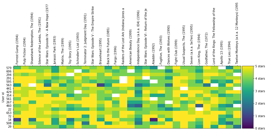
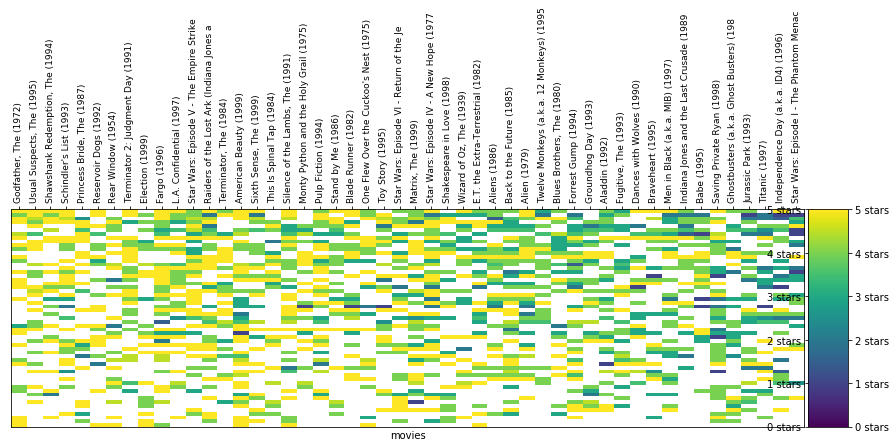
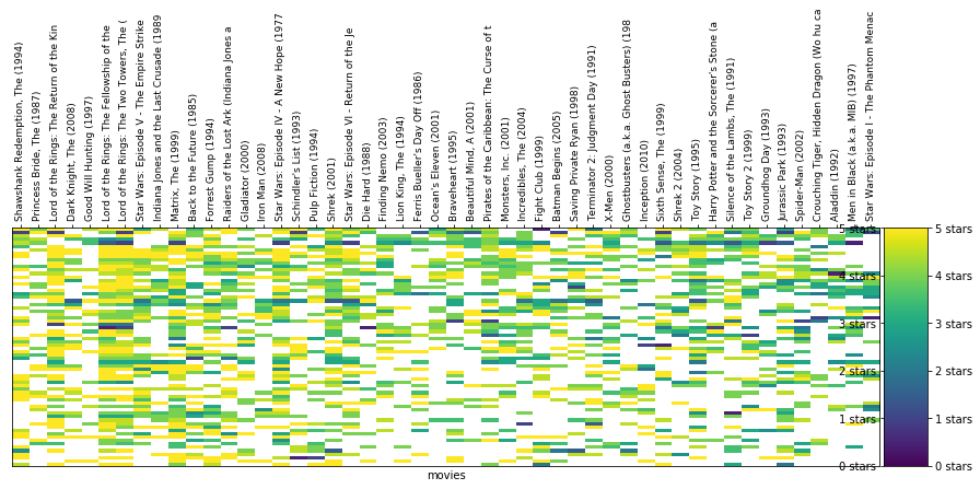
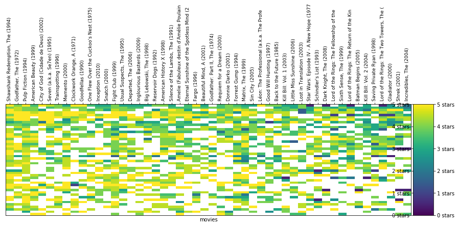
每列表示一部电影。每行表示一位用户。单元格的颜色根据图表右侧的刻度表示用户对该电影的评分情况。 注意到某些单元格是白色吗?表示相应用户没有对该电影进行评分。在现实中进行聚类时就会遇到这种问题。与一开始经过整理的示例不同,现实中的数据集经常比较稀疏,数据集中的部分单元格没有值。这样的话,直接根据电影评分对用户进行聚类不太方便,因为 k 均值通常不喜欢缺失值。 4.2.2 稀疏 csr 矩阵为了提高性能,我们将仅使用 1000 部电影的评分(数据集中一共有 9000 部以上)。 user_movie_ratings = pd.pivot_table(ratings_title, index='userId', columns= 'title', values='rating') most_rated_movies_1k = helper.get_most_rated_movies(user_movie_ratings, 1000)为了使 sklearn 对像这样缺少值的数据集运行 k 均值聚类,我们首先需要将其转型为稀疏 csr 矩阵类型(如 SciPi 库中所定义)。 要从 pandas dataframe 转换为稀疏矩阵,我们需要先转换为 SparseDataFrame,然后使用 pandas 的 to_coo() 方法进行转换。 注意:只有较新版本的 pandas 具有to_coo()。 将dataframe 转换为稀疏矩阵并进行聚类(随意选取 K=20,选择 k 的更佳方式如上述肘部方法所示。但是,该方法需要一定的运行时间),为了可视化其中一些聚类,我们将每个聚类绘制成热图: sparse_ratings = csr_matrix(pd.SparseDataFrame(most_rated_movies_1k).to_coo()) predictions = KMeans(n_clusters=20, algorithm='full').fit_predict(sparse_ratings) max_users = 70 max_movies = 50 clustered = pd.concat([most_rated_movies_1k.reset_index(), pd.DataFrame({'group':predictions})], axis=1) helper.draw_movie_clusters(clustered, max_users, max_movies) cluster # 2 # of users in cluster: 257. # of users in plot: 70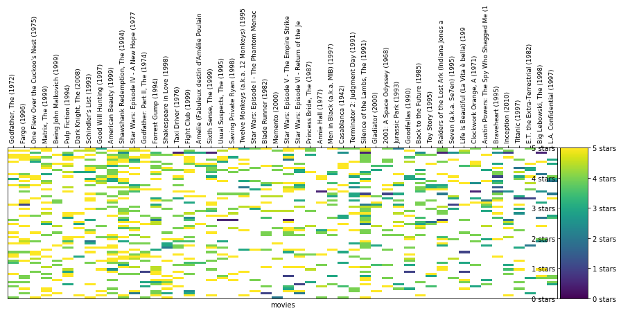 cluster # 13
# of users in cluster: 74. # of users in plot: 70
cluster # 13
# of users in cluster: 74. # of users in plot: 70
 cluster # 14
# of users in cluster: 57. # of users in plot: 57
cluster # 14
# of users in cluster: 57. # of users in plot: 57
 cluster # 18
# of users in cluster: 80. # of users in plot: 70
cluster # 18
# of users in cluster: 80. # of users in plot: 70
 cluster # 3
# of users in cluster: 46. # of users in plot: 46
cluster # 3
# of users in cluster: 46. # of users in plot: 46
 cluster # 16
# of users in cluster: 37. # of users in plot: 37
cluster # 16
# of users in cluster: 37. # of users in plot: 37
 cluster # 5
# of users in cluster: 22. # of users in plot: 22
cluster # 5
# of users in cluster: 22. # of users in plot: 22
 cluster # 12
# of users in cluster: 33. # of users in plot: 33
cluster # 12
# of users in cluster: 33. # of users in plot: 33
 cluster # 9
# of users in cluster: 22. # of users in plot: 22
cluster # 9
# of users in cluster: 22. # of users in plot: 22
需要注意以下几个事项: 聚类中的评分越相似,你在该聚类中就越能发现颜色相似的垂直线。在聚类中发现了非常有趣的规律:某些聚类比其他聚类更稀疏,其中的用户可能比其他聚类中的用户看的电影更少,评分的电影也更少。某些聚类主要是黄色,汇聚了非常喜欢特定类型电影的用户。其他聚类主要是绿色或海蓝色,表示这些用户都认为某些电影可以评 2-3 颗星。注意每个聚类中的电影有何变化。图表对数据进行了过滤,仅显示评分最多的电影,然后按照平均评分排序。很容易发现具有相似颜色的水平线,表示评分变化不大的用户。这可能是 Netflix 从基于星级的评分切换到喜欢/不喜欢评分的原因之一。四颗星评分对不同的人来说,含义不同。我们在可视化聚类时,采取了一些措施(过滤/排序/切片)。因为这种数据集比较“稀疏”,大多数单元格没有值(因为大部分用户没有看过大部分电影)。 4.2.3 利用聚类结果进行预测我们选择一个聚类和一位特定的用户,看看该聚类可以使我们执行哪些实用的操作。 首先选择一个聚类: # TODO: Pick a cluster ID from the clusters above cluster_number = 11 # Let's filter to only see the region of the dataset with the most number of values n_users = 75 n_movies = 300 cluster = clustered[clustered.group == cluster_number].drop(['index', 'group'], axis=1) cluster = helper.sort_by_rating_density(cluster, n_movies, n_users) helper.draw_movies_heatmap(cluster, axis_labels=False)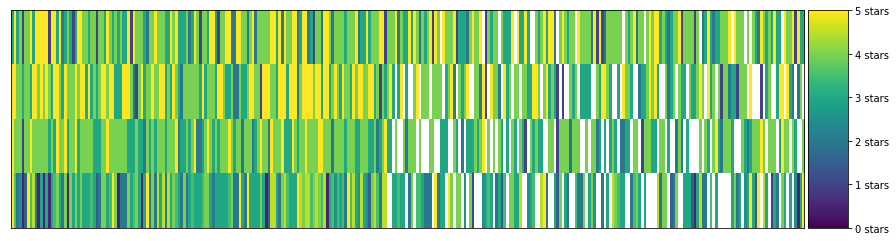
聚类中的实际评分如下所示: cluster.fillna('').head() Forrest Gump (1994)Sixteen Candles (1984)Wizard of Oz, The (1939)Mummy, The (1999)Congo (1995)First Wives Club, The (1996)West Side Story (1961)Sting, The (1973)Sound of Music, The (1965)Stand by Me (1986)...What's Eating Gilbert Grape (1993)When Harry Met Sally... (1989)North by Northwest (1959)Breakfast Club, The (1985)Casablanca (1942)Big Lebowski, The (1998)Mr. Holland's Opus (1995)Nightmare Before Christmas, The (1993)Broken Arrow (1996)Four Weddings and a Funeral (1994)33.05.03.04.01.04.04.05.03.05.0...35445153325.05.04.04.03.04.04.03.05.05.0...555322405.04.04.04.01.04.04.05.04.04.0...354443415.03.52.02.50.51.55.03.54.52.0...4332.50.5354 rows × 300 columns 从表格中选择一个空白单元格。因为用户没有对该电影评分,所以是空白状态。 因为该用户属于似乎具有相似品位的用户聚类,我们可以计算该电影在此聚类中的平均评分,结果可以作为她是否喜欢电影 “Forrest Gump (1994)” 的合理预测依据。 # TODO: Fill in the name of the column/movie. e.g. 'Forrest Gump (1994)' movie_name = "Forrest Gump (1994)" cluster[movie_name].mean() 4.5这就是我们关于她会如何对该电影进行评分的预测。 4.2.4 利用聚类结果进行推荐我们回顾下上一步的操作。我们使用 k 均值根据用户的评分对用户进行聚类。这样就形成了具有相似评分的用户聚类,因此通常具有相似的电影品位。基于这一点,当某个用户对某部电影没有评分时,我们对该聚类中所有其他用户的评分取平均值,该平均值就是我们猜测该用户对该电影的喜欢程度。 根据这一逻辑,如果我们计算该聚类中每部电影的平均分数,就可以判断该“品位聚类”对数据集中每部电影的喜欢程度。 # The average rating of 20 movies as rated by the users in the cluster cluster.mean().head(20) Forrest Gump (1994) 4.500 Sixteen Candles (1984) 4.375 Wizard of Oz, The (1939) 3.250 Mummy, The (1999) 3.625 Congo (1995) 1.375 First Wives Club, The (1996) 3.375 West Side Story (1961) 4.250 Sting, The (1973) 4.125 Sound of Music, The (1965) 4.125 Stand by Me (1986) 4.000 Heathers (1989) 3.375 Victor/Victoria (1982) 4.250 Sex, Lies, and Videotape (1989) 3.375 Pulp Fiction (1994) 4.250 Outbreak (1995) 2.125 Jaws (1975) 3.750 Who Framed Roger Rabbit? (1988) 4.125 Big (1988) 4.250 Romy and Michele's High School Reunion (1997) 4.000 Forget Paris (1995) 2.750 dtype: float64这对我们来说变得非常实用,因为现在我们可以使用它作为推荐引擎,使用户能够发现他们可能喜欢的电影。 当用户登录我们的应用时,现在我们可以向他们显示符合他们的兴趣品位的电影。推荐方式是选择聚类中该用户尚未评分的最高评分的电影。、 |
【本文地址】