【机器学习】python实现非线性回归（以中国1960

您所在的位置：网站首页 › 多元非线性回归预测模型建模 › 【机器学习】python实现非线性回归（以中国1960

【机器学习】python实现非线性回归（以中国1960

#【机器学习】python实现非线性回归（以中国1960| 来源: 网络整理| 查看: 265

非线性回归目标区分线性回归和非线性回归用py实现非线性回归

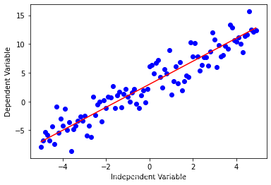
如果数据表现出一个曲线的趋势，那么相比于非线性回归，线性回归就不会产生一个非常精确的结果，因为线性回归假设数据是线性的。就让我们通过一个例子学习一下非线性回归。在这篇博客中我们对中国1960年到2014年的GDP拟合了一个非线性模型。

导入相关库 import numpy as np import matplotlib.pyplot as plt %matplotlib inline

虽然线性回归在有的数据集上表现的很好，但是它不能应用到所有数据集。首先我们回想一下线性回归，它是拟合因变量y和自变量x，方程是很简单的，比如 y = 2 x + 3 y = 2x + 3 y=2x+3。

下面用代码来看看。

x = np.arange(-5.0, 5.0, 0.1) ##You can adjust the slope and intercept to verify the changes in the graph y = 2*(x) + 3 y_noise = 2 * np.random.normal(size=x.size) ydata = y + y_noise #plt.figure(figsize=(8,6)) plt.plot(x, ydata, 'bo') plt.plot(x,y, 'r') plt.ylabel('Dependent Variable') plt.xlabel('Independent Variable') plt.show()

请添加图片描述

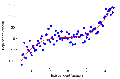
非线性回归是用一种拟合自变量 x x x 和因变量 y y y之间的非线性关系的一种方法。

比如下面是一个多项式。

y = a x 3 + b x 2 + c x + d \ y = a x^3 + b x^2 + c x + d \ y=ax3+bx2+cx+d

非线性函数有指数、对数、分数等元素

y = log ⁡ ( x ) y = \log(x) y=log(x)

也可以是这种复杂的形式 y = log ⁡ ( a x 3 + b x 2 + c x + d ) y = \log(a x^3 + b x^2 + c x + d) y=log(ax3+bx2+cx+d)

让我们看看这个三次函数

x = np.arange(-5.0, 5.0, 0.1) ##You can adjust the slope and intercept to verify the changes in the graph y = 1*(x**3) + 1*(x**2) + 1*x + 3 # 加点噪音，也就是随机数 y_noise = 20 * np.random.normal(size=x.size) ydata = y + y_noise plt.plot(x, ydata, 'bo') plt.plot(x,y, 'r') plt.ylabel('Dependent Variable') plt.xlabel('Independent Variable') plt.show()

在这里插入图片描述

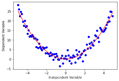
还有一些其他的形式

二次函数

Y = X 2 Y = X^2 Y=X2

x = np.arange(-5.0, 5.0, 0.1) ##You can adjust the slope and intercept to verify the changes in the graph y = np.power(x,2) y_noise = 2 * np.random.normal(size=x.size) ydata = y + y_noise plt.plot(x, ydata, 'bo') plt.plot(x,y, 'r') plt.ylabel('Dependent Variable') plt.xlabel('Independent Variable') plt.show()

在这里插入图片描述

指数函数

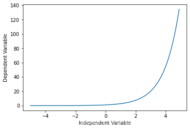
Y = a + b c X Y = a + b c^X Y=a+bcX 其中 b ≠ 0 , c > 0 , c ≠ 1 其中b ≠0, c > 0 , c ≠1 其中b=0,c>0,c=1

X = np.arange(-5.0, 5.0, 0.1) ##You can adjust the slope and intercept to verify the changes in the graph Y= np.exp(X) plt.plot(X,Y) plt.ylabel('Dependent Variable') plt.xlabel('Independent Variable') plt.show()

在这里插入图片描述

对数

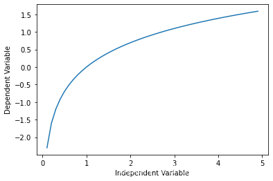
y = log ⁡ ( x ) y = \log(x) y=log(x)

X = np.arange(-5.0, 5.0, 0.1) Y = np.log(X) plt.plot(X,Y) plt.ylabel('Dependent Variable') plt.xlabel('Independent Variable') plt.show()

在这里插入图片描述

Sigmoidal/Logistic

Y = a + b 1 + c ( X − d ) Y = a + \frac{b}{1+ c^{(X-d)}} Y=a+1+c(X−d)b

X = np.arange(-5.0, 5.0, 0.1) Y = 1-4/(1+np.power(3, X-2)) plt.plot(X,Y) plt.ylabel('Dependent Variable') plt.xlabel('Independent Variable') plt.show()

在这里插入图片描述

非线性回归的例子

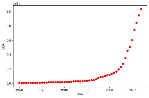
我们将要拟合中国从1960年到2014年的GDP数据。我们下载的数据有两列，第一列是年份，从1960到2014，第二列是对应年份的国内生产总值（美元）。

gdp数据（点我下载(❁´◡`❁)）

import numpy as np import pandas as pd df = pd.read_csv("china_gdp.csv") df.head(10) YearValue019605.918412e+10119614.955705e+10219624.668518e+10319635.009730e+10419645.906225e+10519656.970915e+10619667.587943e+10719677.205703e+10819686.999350e+10919697.871882e+10 数据可视化

数据有点像logistic或者指数函数，一开始增长得特别慢，从2005年开始，增长速度就非常显著了，在2010年代略微减速。

plt.figure(figsize=(8,5)) x_data, y_data = (df["Year"].values, df["Value"].values) plt.plot(x_data, y_data, 'ro') # plt.stem(x_data, y_data) plt.ylabel('GDP') plt.xlabel('Year') plt.show()

在这里插入图片描述

选择模型

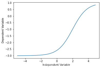
从第一眼看这个散点图，我就感觉logistic函数会不错，因为一开始增长很慢、中间增长很快、最后又慢了下来

就像下面这样：

X = np.arange(-5.0, 5.0, 0.1) Y = 1.0 / (1.0 + np.exp(-X)) plt.plot(X,Y) plt.ylabel('Dependent Variable') plt.xlabel('Independent Variable') plt.show()

[外链图片转存失败,源站可能有防盗链机制,建议将图片保存下来直接上传(img-7EHjyekz-1655197597832)(output_28_0.png)]

logsitic函数的方程如下

Y ^ = 1 1 + e − β _ 1 ( X − β _ 2 ) \hat{Y} = \frac1{1+e^{-\beta\_1(X-\beta\_2)}} Y^=1+e−β_1(X−β_2)1

β _ 1 \beta\_1 β_1: 控制曲线的陡度,

β _ 2 \beta\_2 β_2: x轴上平移

构建模型

现在，让我们构建我们的回归模型并且初始化参数

def sigmoid(x, Beta_1, Beta_2): y = 1 / (1 + np.exp(-Beta_1*(x-Beta_2))) return y

首先随便搞两个参数

beta_1 = 0.10 beta_2 = 1990.0 #logistic function Y_pred = sigmoid(x_data, beta_1 , beta_2) #plot initial prediction against datapoints plt.plot(x_data, Y_pred*15000000000000.) plt.plot(x_data, y_data, 'ro')

[外链图片转存失败,源站可能有防盗链机制,建议将图片保存下来直接上传(img-fdiZTFbv-1655197597833)(output_33_1.png)]

我们的目标是找到最好的参数。

第一步把x和y都标准化一下。

# Lets normalize our data xdata =x_data/max(x_data) ydata =y_data/max(y_data) 如何找到拟合曲线最好的参数？

我们可以使用curve_fit，它使用非线性最小二乘来拟合我们的sigmoid函数。优化参数值，使sigmoid(xdata， *popt) - ydata的残差平方和最小化。

Popt是我们的优化参数。

from scipy.optimize import curve_fit popt, pcov = curve_fit(sigmoid, xdata, ydata) #print the final parameters print(" beta_1 = %f, beta_2 = %f" % (popt[0], popt[1])) beta_1 = 690.451711, beta_2 = 0.997207

现在画一下我们的回归模型。

x = np.linspace(1960, 2015, 55) x = x/max(x) plt.figure(figsize=(8,5)) y = sigmoid(x, *popt) plt.plot(xdata, ydata, 'ro', label='data') plt.plot(x,y, linewidth=3.0, label='fit') plt.legend(loc='best') plt.ylabel('GDP') plt.xlabel('Year') plt.show()

[外链图片转存失败,源站可能有防盗链机制,建议将图片保存下来直接上传(img-PIAwrPIA-1655197597833)(output_39_0.png)]

评估模型

虽然看上去不错，但是在运行过程中 R 2 R^2 R2有时竟是负的，而且就是 R 2 R^2 R2很大的时候在测试集上实际效果也不是很好，所以还是不很靠谱。

# 把数据分为训练集和测试集 msk=np.random.rand(len(df))

【本文地址】

公司简介

联系我们