| 时序分析 19 VAR(Vector Autoregression) 向量自回归 | 您所在的位置:网站首页 › 多元时间序列预测是什么 › 时序分析 19 VAR(Vector Autoregression) 向量自回归 |
时序分析 19 VAR(Vector Autoregression) 向量自回归
|
时序分析 19 向量自回归 (VAR)
VAR (Vector Autoregressive)
简介
本文开始介绍VAR(Vector Autoregressive)向量自回归。 前面我们讨论了多个自回归模型,例如AR, ARMA, ARIMA等。而向量自回归和已讨论地自回归模型有本质的区别:类似AR等模型所建模的关系都是单向的,而VAR是双向的。 所谓单向就是模型的关系是一个方向,就是历史的情况影响现在的情况而现在是不能影响历史的;而VAR建模需要2个或者更多的时序变量,这些时序变量的影响是双向的。一个变量影响另一个的同时,这个变量也受到另一个的影响。 VAR的自回归就是指一个时序变量的值是该变量本身过去的值和其他变量过去的值的线性函数。 理论 先看一下公式让我们有一个直观理解,例如我们有两个时序变量
Y
1
Y_1
Y1 和
Y
2
Y_2
Y2,模型
V
A
R
(
2
)
VAR(2)
VAR(2) 可以表示为
Y
1
,
t
=
α
1
+
β
11
,
1
Y
1
,
t
−
1
+
β
12
,
1
Y
2
,
t
−
1
+
β
11
,
2
Y
1
,
t
−
2
+
β
12
,
2
Y
2
,
t
−
2
+
ϵ
1
,
t
Y_{1,t}=\alpha_1+\beta_{11,1}Y_{1,t-1}+\beta_{12,1}Y_{2,t-1}+\beta_{11,2}Y_{1,t-2}+\beta_{12,2}Y_{2,t-2}+\epsilon_{1,t}
Y1,t=α1+β11,1Y1,t−1+β12,1Y2,t−1+β11,2Y1,t−2+β12,2Y2,t−2+ϵ1,t
Y
2
,
t
=
α
2
+
β
21
,
1
Y
1
,
t
−
1
+
β
22
,
1
Y
2
,
t
−
1
+
β
21
,
2
Y
1
,
t
−
2
+
β
22
,
2
Y
2
,
t
−
2
+
ϵ
2
,
t
Y_{2,t}=\alpha_2+\beta_{21,1}Y_{1,t-1}+\beta_{22,1}Y_{2,t-1}+\beta_{21,2}Y_{1,t-2}+\beta_{22,2}Y_{2,t-2}+\epsilon_{2,t}
Y2,t=α2+β21,1Y1,t−1+β22,1Y2,t−1+β21,2Y1,t−2+β22,2Y2,t−2+ϵ2,t
V
A
R
(
2
)
VAR(2)
VAR(2) 即2阶
V
A
R
VAR
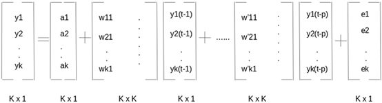
VAR 模型 不难得出,k个时序变量p阶形式可以表示为 数据集各字段的含义如下: rgnp : Real GNP. 真实国民生产总值pgnp : Potential real GNP. 潜在真实国民生产总值ulc : Unit labor cost. 单位劳动力成本gdfco : Fixed weight deflator for personal consumption expenditure excluding food and energy. 剔除食物和能源的个人消费支出的固定权重平减指数gdf : Fixed weight GNP deflator. 固定权重GNP平减指数。gdfim : Fixed weight import deflator. 固定权重进口平减指数gdfcf : Fixed weight deflator for food in personal consumption expenditure.个人食物消费支出的固定权重平减指数gdfce : Fixed weight deflator for energy in personal consumption expenditure.个人能源消费支出的固定权重平减指数 #filepath = 'https://raw.githubusercontent.com/selva86/datasets/master/Raotbl6.csv' df = pd.read_csv("Raotbl6.csv", parse_dates=['date'], index_col='date') print(df.shape) # (123, 8) df.tail()
VAR背后的逻辑是这些时序变量是互相影响的,也就是说一个时序变量的变化是由其他时序变量引起的。所以检验是否存在一定的因果关系是应用VAR模型的先决条件。 这里我们将采用Granger’s Causality Test。 Granger’s Causality Test的原假设是回归方程中所有过去的值的系数都为0.简单来说,如果时序X的过去的值并不能影响另一个时序Y.如果p-value小于0.05的显著性水平,就可以拒绝原假设。 from statsmodels.tsa.stattools import grangercausalitytests maxlag=12 test = 'ssr_chi2test' def grangers_causation_matrix(data, variables, test='ssr_chi2test', verbose=False): """Check Granger Causality of all possible combinations of the Time series. The rows are the response variable, columns are predictors. The values in the table are the P-Values. P-Values lesser than the significance level (0.05), implies the Null Hypothesis that the coefficients of the corresponding past values is zero, that is, the X does not cause Y can be rejected. data : pandas dataframe containing the time series variables variables : list containing names of the time series variables. """ df = pd.DataFrame(np.zeros((len(variables), len(variables))), columns=variables, index=variables) for c in df.columns: for r in df.index: test_result = grangercausalitytests(data[[r, c]], maxlag=maxlag, verbose=False) p_values = [round(test_result[i+1][0][test][1],4) for i in range(maxlag)] if verbose: print(f'Y = {r}, X = {c}, P Values = {p_values}') min_p_value = np.min(p_values) df.loc[r, c] = min_p_value df.columns = [var + '_x' for var in variables] df.index = [var + '_y' for var in variables] return df grangers_causation_matrix(df, variables = df.columns)
注:关于协整序列的定义和相关概念,请参见本系列文章协整序列 from statsmodels.tsa.vector_ar.vecm import coint_johansen def cointegration_test(df, alpha=0.05): """Perform Johanson's Cointegration Test and Report Summary""" out = coint_johansen(df,-1,5) d = {'0.90':0, '0.95':1, '0.99':2} traces = out.lr1 cvts = out.cvt[:, d[str(1-alpha)]] def adjust(val, length= 6): return str(val).ljust(length) # Summary print('Name :: Test Stat > C(95%) => Signif \n', '--'*20) for col, trace, cvt in zip(df.columns, traces, cvts): print(adjust(col), ':: ', adjust(round(trace,2), 9), ">", adjust(cvt, 8), ' => ' , trace > cvt) cointegration_test(df)
VAR模型需要参与的时序是平稳的。 def adfuller_test(series, signif=0.05, name='', verbose=False): """Perform ADFuller to test for Stationarity of given series and print report""" r = adfuller(series, autolag='AIC') output = {'test_statistic':round(r[0], 4), 'pvalue':round(r[1], 4), 'n_lags':round(r[2], 4), 'n_obs':r[3]} p_value = output['pvalue'] def adjust(val, length= 6): return str(val).ljust(length) # Print Summary print(f' Augmented Dickey-Fuller Test on "{name}"', "\n ", '-'*47) print(f' Null Hypothesis: Data has unit root. Non-Stationary.') print(f' Significance Level = {signif}') print(f' Test Statistic = {output["test_statistic"]}') print(f' No. Lags Chosen = {output["n_lags"]}') for key,val in r[4].items(): print(f' Critical value {adjust(key)} = {round(val, 3)}') if p_value 4 # Input data for forecasting forecast_input = df_differenced.values[-lag_order:] forecast_input4 array([[ 13.5, 0.1, 1.4, 0.1, 0.1, -0.1, 0.4, -2. ], [-23.6, 0.2, -2. , -0.5, -0.1, -0.2, -0.3, -1.2], [ -3.3, 0.1, 3.1, 0.5, 0.3, 0.4, 0.9, 2.2], [ -3.9, 0.2, -2.1, -0.4, 0.2, -1.5, 0.9, -0.3]]) # Forecast fc = model_fitted.forecast(y=forecast_input, steps=nobs) df_forecast = pd.DataFrame(fc, index=df.index[-nobs:], columns=df.columns + '_2d') df_forecast
本篇文章以理论结合实践的方式系统介绍了VAR时序建模技术,中间还涉及了其他一些其他关联技术,例如因果测试、协整测试、序列相关测试等。在整个过程中,还包含了平稳过程的测试、如何找到最佳的阶数P、样本划分、差分等。 大家可以看到,一个完整的时序分析过程是非常复杂的,它牵涉到许多相关的模型技术和知识、数据分析技术等。希望大家读完这篇文章,能对时序数据的分析过程有一个概要了解。 需要提醒大家的是,真正的技术永远是自己做出来的而不可能从书本上学到。 |

 大部分都有上升趋势,但gdfim和gdfce略有不同
 以上对时序的所有可能组合都进行了检验。结果中记录的就是p-value,所有p-value都小于0.05。所以目前我们在0.05的显著性水平上拒绝原假设,所有时序之间都是存在关系的。也就是说,VAR模型可能很适合解释这个数据集中的时序数据关系。
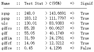 协整关系说明两个时序具有长期的统计上的关系,这正符合VAR的假设。
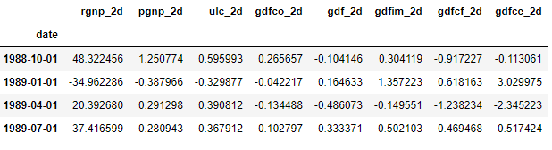 得到的结果是二阶差分的结果,我们需要做逆向。
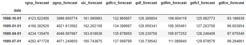
 检验和评价预测结果,我们将计算MAPE, ME, MAE, MPE, RMSE, corr 和 minmax
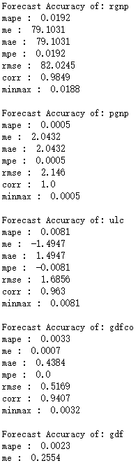 …省略
…省略【本文地址】