| R语言绘制研究区概况图 | 您所在的位置:网站首页 › 北宋行政区划地图 › R语言绘制研究区概况图 |
R语言绘制研究区概况图
|
之前用R语言绘图一直用的是tmap包,今天试了试ggplot2包,效果还可以但没用达到自己的预期,记录在知乎方便自己复现(读者朋友有好的绘图方法也可以分享给我)~ 效果如下:  一、绘制左边的标准中国地图(研究区用橙色填充)# 加载包
library(sf)
library(stars)
library(terra)
library(ggspatial)
library(tidyverse)读取中国省级行政区划数据和九段线数据并设置投影为阿尔伯斯等积投影# 绘制中国地图常用的Albers Equal Area Conic投影
albers = "+proj=aea +lat_1=25 +lat_2=47 +lon_0=105"
# 读取中国省级行政区划数据和九段线数据并设置投影为阿尔伯斯等积投影
province = read_sf('./data/province.geojson') |>
st_transform(st_crs(albers))
nineline = read_sf('./data/nineline.geojson') |>
st_transform(st_crs(albers)) 一、绘制左边的标准中国地图(研究区用橙色填充)# 加载包
library(sf)
library(stars)
library(terra)
library(ggspatial)
library(tidyverse)读取中国省级行政区划数据和九段线数据并设置投影为阿尔伯斯等积投影# 绘制中国地图常用的Albers Equal Area Conic投影
albers = "+proj=aea +lat_1=25 +lat_2=47 +lon_0=105"
# 读取中国省级行政区划数据和九段线数据并设置投影为阿尔伯斯等积投影
province = read_sf('./data/province.geojson') |>
st_transform(st_crs(albers))
nineline = read_sf('./data/nineline.geojson') |>
st_transform(st_crs(albers))展示一下上一步读取的省级行政区划和九段线数据 plot(province[1])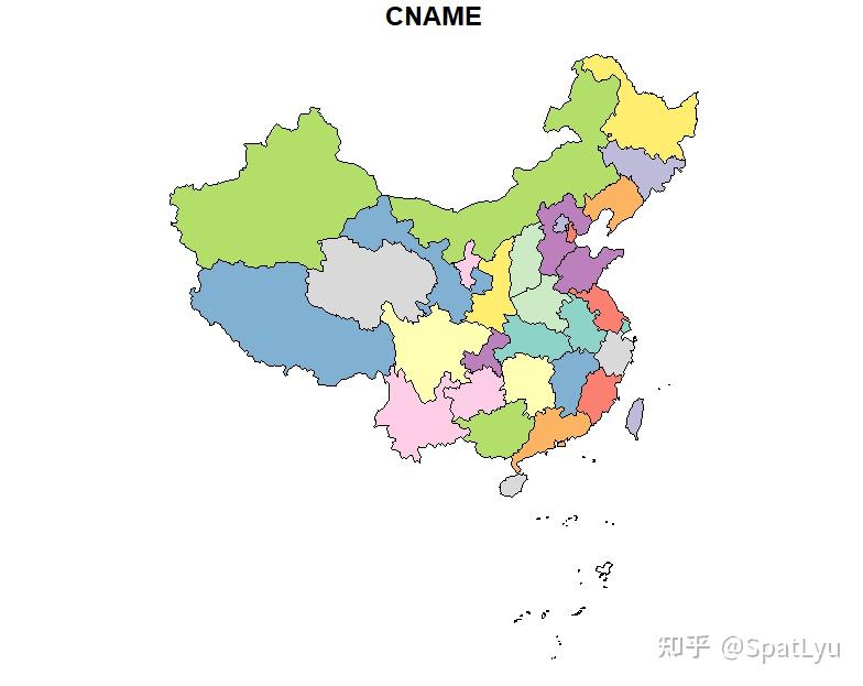 plot(nineline[1]) plot(nineline[1]) 合并省级行政区划和九段线province = st_union(province,nineline)绘制大图fig1 = ggplot() +
geom_sf(size = .2, fill = "transparent", color = "#060d1b", data=province)
fig1 合并省级行政区划和九段线province = st_union(province,nineline)绘制大图fig1 = ggplot() +
geom_sf(size = .2, fill = "transparent", color = "#060d1b", data=province)
fig1 绘制南海小地图:fig2 = fig1+
coord_sf(crs = st_crs('epsg:4326')) + ## 将投影坐标转换为大地坐标
scale_x_continuous(expand = c(0, 0), limits = c(107, 122), breaks = seq(70, 140, 10)) +
scale_y_continuous(expand = c(0, 0), limits = c(2, 24), breaks = seq(10, 60, 10)) +
guides(fill = "none", color = "none") +
theme_bw() +
theme(
axis.text = element_blank(),
axis.ticks = element_blank(),
axis.title = element_blank()
)
fig2 绘制南海小地图:fig2 = fig1+
coord_sf(crs = st_crs('epsg:4326')) + ## 将投影坐标转换为大地坐标
scale_x_continuous(expand = c(0, 0), limits = c(107, 122), breaks = seq(70, 140, 10)) +
scale_y_continuous(expand = c(0, 0), limits = c(2, 24), breaks = seq(10, 60, 10)) +
guides(fill = "none", color = "none") +
theme_bw() +
theme(
axis.text = element_blank(),
axis.ticks = element_blank(),
axis.title = element_blank()
)
fig2 读取渭河流域边界矢量数据并转换投影至阿尔伯斯投影:weihe = read_sf('./data/渭河流域边界/') |>
st_transform(st_crs(albers))
plot(weihe[1]) 读取渭河流域边界矢量数据并转换投影至阿尔伯斯投影:weihe = read_sf('./data/渭河流域边界/') |>
st_transform(st_crs(albers))
plot(weihe[1]) 拼接大图和南海小地图并对渭河流域地区填充颜色:fig1 +
geom_sf(data=weihe,size = 3.5,
fill = "#FDBF6F", color = "#E31A1C")+
coord_sf(crs = st_crs(albers), default_crs = st_crs('epsg:4326')) +
scale_x_continuous(expand = c(0, 0),
limits=c(72,142),
breaks=seq(70, 140, 10)) +
scale_y_continuous(expand = c(0, 0),
limits = c(17,55.5),
breaks = seq(10, 60, 10)) +
theme_bw() +
theme(
axis.text = element_text(family ="serif",color="black"),
axis.title = element_blank()) +
annotation_scale(location = "bl") +
annotation_north_arrow(location = "tl", style = north_arrow_nautical(
fill = c("grey40", "white"), line_col = "grey20")) +
annotation_custom(ggplotGrob(fig2),
xmin= 122,xmax = 138,
ymin=15,ymax = 29) -> total.china
total.china 拼接大图和南海小地图并对渭河流域地区填充颜色:fig1 +
geom_sf(data=weihe,size = 3.5,
fill = "#FDBF6F", color = "#E31A1C")+
coord_sf(crs = st_crs(albers), default_crs = st_crs('epsg:4326')) +
scale_x_continuous(expand = c(0, 0),
limits=c(72,142),
breaks=seq(70, 140, 10)) +
scale_y_continuous(expand = c(0, 0),
limits = c(17,55.5),
breaks = seq(10, 60, 10)) +
theme_bw() +
theme(
axis.text = element_text(family ="serif",color="black"),
axis.title = element_blank()) +
annotation_scale(location = "bl") +
annotation_north_arrow(location = "tl", style = north_arrow_nautical(
fill = c("grey40", "white"), line_col = "grey20")) +
annotation_custom(ggplotGrob(fig2),
xmin= 122,xmax = 138,
ymin=15,ymax = 29) -> total.china
total.china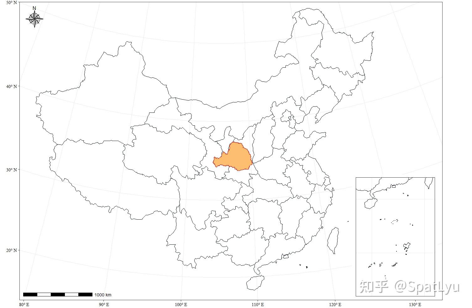 二、绘制右边以NDVI作底图的渭河流域研究区图读取相应的地理矢量数据:weihe_boundry = read_sf('./data/渭河流域边界/')
river1 = read_sf('./data/weihebasin_rivers/river3.shp') |> vect() |> st_as_sf()
river2 = read_sf('./data/weihebasin_rivers/river4.shp') |> vect() |> st_as_sf()
river3 = read_sf('./data/weihebasin_rivers/river5.shp') |> vect() |> st_as_sf()
citypoint = read_sf('./data/省市县-湖泊/地级市渭河流域_point.shp')|>
vect() |> st_as_sf()作为底图的NDVI数据的裁切和格式转换:ndvi = terra::rast('./data/image/ndvi.tif') |>
terra::crop(terra::vect(weihe_boundry),mask=T) |>
st_as_stars() |>
st_as_sf()定义绘制NDVI底图时的色带:colors = c('#d73027',
'#f46d43',
'#fdae61',
'#fee08b',
'#d9ef8b',
'#a6d96a',
'#66bd63',
'#1a9850') 二、绘制右边以NDVI作底图的渭河流域研究区图读取相应的地理矢量数据:weihe_boundry = read_sf('./data/渭河流域边界/')
river1 = read_sf('./data/weihebasin_rivers/river3.shp') |> vect() |> st_as_sf()
river2 = read_sf('./data/weihebasin_rivers/river4.shp') |> vect() |> st_as_sf()
river3 = read_sf('./data/weihebasin_rivers/river5.shp') |> vect() |> st_as_sf()
citypoint = read_sf('./data/省市县-湖泊/地级市渭河流域_point.shp')|>
vect() |> st_as_sf()作为底图的NDVI数据的裁切和格式转换:ndvi = terra::rast('./data/image/ndvi.tif') |>
terra::crop(terra::vect(weihe_boundry),mask=T) |>
st_as_stars() |>
st_as_sf()定义绘制NDVI底图时的色带:colors = c('#d73027',
'#f46d43',
'#fdae61',
'#fee08b',
'#d9ef8b',
'#a6d96a',
'#66bd63',
'#1a9850')绘制渭河流域区域图: ggplot() + geom_sf(aes(fill=NDVI_mean,color=NDVI_mean),data=ndvi) + geom_sf(data = river1,lwd = 1, fill = "transparent", color = "#045a8d")+ geom_sf(data = river2,lwd = 0.6, fill = "transparent", color = "#2b8cbe")+ geom_sf(data = river3,lwd = 0.3, fill = "transparent", color = "#74a9cf")+ scale_fill_gradientn(colours = colors)+ scale_color_gradientn(colours = colors)+ labs(fill = "NDVI", color = "NDVI") + geom_sf_text(data = citypoint, mapping=aes(label = NAME))+ annotation_scale(location = "bl") + annotation_north_arrow(location = "tr", style = north_arrow_nautical( fill = c("grey40", "white"), line_col = "grey20"))+ theme_bw() + theme( panel.grid=element_blank(), legend.position = c(0.15,0.9), legend.justification = c(1,1), axis.text= element_blank(), axis.ticks = element_blank(), axis.title = element_blank() ) -> study.weihe study.weihe 三、将左右图连接到一张图上并导出# 拼接两图
library(patchwork)
fig = total.china+study.weihe
fig 三、将左右图连接到一张图上并导出# 拼接两图
library(patchwork)
fig = total.china+study.weihe
fig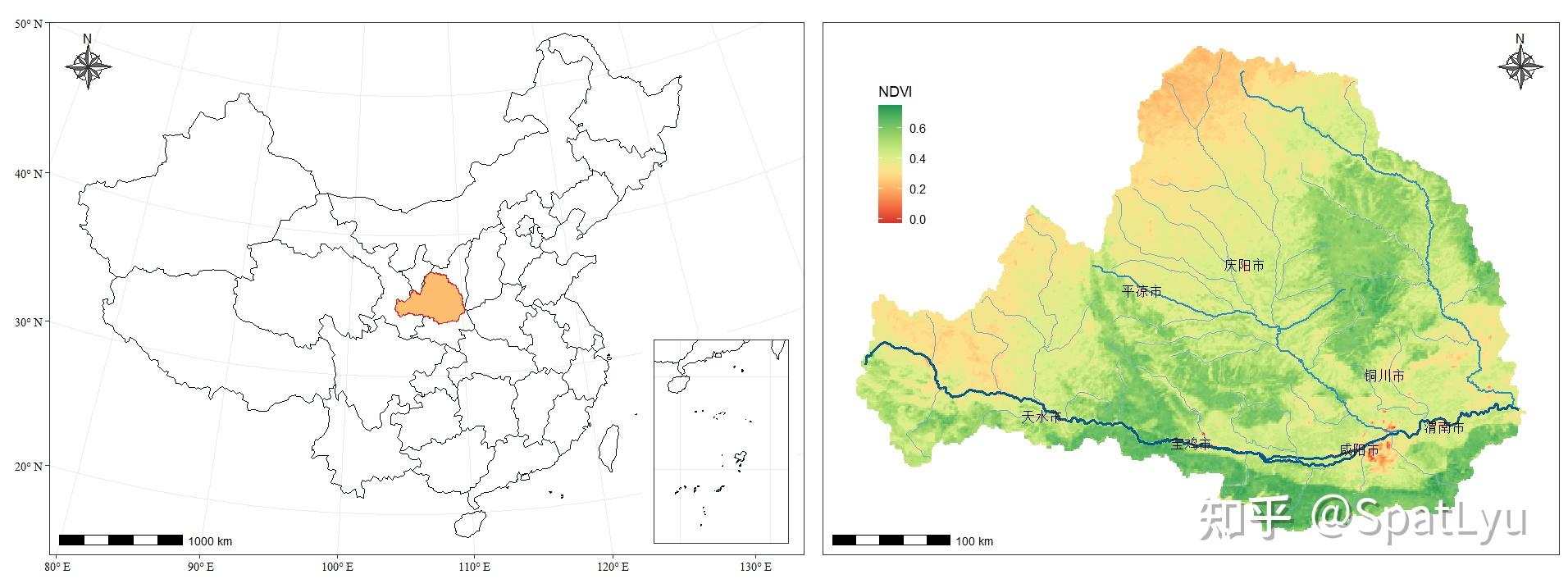 导出绘图结果: ggsave("./figure/study_area.png", fig, width = 15, height = 6, dpi=600)文中用的所有代码如下: # 加载包 library(sf) library(stars) library(terra) library(ggspatial) library(tidyverse) # 绘制中国地图常用的Albers Equal Area Conic投影 albers = "+proj=aea +lat_1=25 +lat_2=47 +lon_0=105" # 读取中国省级行政区划数据和九段线数据并设置投影为阿尔伯斯等积投影 province = read_sf('./data/province.geojson') |> st_transform(st_crs(albers)) nineline = read_sf('./data/nineline.geojson') |> st_transform(st_crs(albers)) # 看一眼 plot(province[1]) plot(nineline[1]) province = st_union(province,nineline) fig1 = ggplot() + geom_sf(size = .2, fill = "transparent", color = "#060d1b", data=province) fig1 fig2 = fig1+ coord_sf(crs = st_crs('epsg:4326')) + ## 将投影坐标转换为大地坐标 scale_x_continuous(expand = c(0, 0), limits = c(107, 122), breaks = seq(70, 140, 10)) + scale_y_continuous(expand = c(0, 0), limits = c(2, 24), breaks = seq(10, 60, 10)) + guides(fill = "none", color = "none") + theme_bw() + theme( axis.text = element_blank(), axis.ticks = element_blank(), axis.title = element_blank() ) fig2 weihe = read_sf('./data/渭河流域边界/') |> st_transform(st_crs(albers)) plot(weihe[1]) fig1 + geom_sf(data=weihe,size = 3.5, fill = "#FDBF6F", color = "#E31A1C")+ coord_sf(crs = st_crs(albers), default_crs = st_crs('epsg:4326')) + scale_x_continuous(expand = c(0, 0), limits=c(72,142), breaks=seq(70, 140, 10)) + scale_y_continuous(expand = c(0, 0), limits = c(17,55.5), breaks = seq(10, 60, 10)) + theme_bw() + theme( axis.text = element_text(family ="serif",color="black"), axis.title = element_blank()) + annotation_scale(location = "bl") + annotation_north_arrow(location = "tl", style = north_arrow_nautical( fill = c("grey40", "white"), line_col = "grey20")) + annotation_custom(ggplotGrob(fig2), xmin= 122,xmax = 138, ymin=15,ymax = 29) -> total.china total.china # 绘制渭河流域研究区域图 weihe_boundry = read_sf('./data/渭河流域边界/') river1 = read_sf('./data/weihebasin_rivers/river3.shp') |> vect() |> st_as_sf() river2 = read_sf('./data/weihebasin_rivers/river4.shp') |> vect() |> st_as_sf() river3 = read_sf('./data/weihebasin_rivers/river5.shp') |> vect() |> st_as_sf() citypoint = read_sf('./data/省市县-湖泊/地级市渭河流域_point.shp')|> vect() |> st_as_sf() coords = st_coordinates(citypoint) citypoint$long = coords[,1] citypoint$lat = coords[,2] ndvi = terra::rast('./data/image/ndvi.tif') |> terra::crop(terra::vect(weihe_boundry),mask=T) |> st_as_stars() |> st_as_sf() colors = c('#d73027', '#f46d43', '#fdae61', '#fee08b', '#d9ef8b', '#a6d96a', '#66bd63', '#1a9850') ggplot() + geom_sf(aes(fill=NDVI_mean,color=NDVI_mean),data=ndvi) + geom_sf(data = river1,lwd = 1, fill = "transparent", color = "#045a8d")+ geom_sf(data = river2,lwd = 0.6, fill = "transparent", color = "#2b8cbe")+ geom_sf(data = river3,lwd = 0.3, fill = "transparent", color = "#74a9cf")+ scale_fill_gradientn(colours = colors)+ scale_color_gradientn(colours = colors)+ labs(fill = "NDVI", color = "NDVI") + geom_sf_text(data = citypoint, mapping=aes(x = long, y = lat, label = NAME))+ annotation_scale(location = "bl") + annotation_north_arrow(location = "tr", style = north_arrow_nautical( fill = c("grey40", "white"), line_col = "grey20"))+ theme_bw() + theme( panel.grid=element_blank(), legend.position = c(0.15,0.9), legend.justification = c(1,1), axis.text= element_blank(), axis.ticks = element_blank(), axis.title = element_blank() ) -> study.weihe study.weihe # 拼接两图 library(patchwork) fig = total.china+study.weihe fig ggsave("./figure/study_area.png", fig, width = 15, height = 6, dpi=600)# 加载包 library(sf) library(stars) library(terra) library(ggspatial) library(tidyverse) # 绘制中国地图常用的Albers Equal Area Conic投影 albers = "+proj=aea +lat_1=25 +lat_2=47 +lon_0=105" # 读取中国省级行政区划数据和九段线数据并设置投影为阿尔伯斯等积投影 province = read_sf('./data/province.geojson') |> st_transform(st_crs(albers)) nineline = read_sf('./data/nineline.geojson') |> st_transform(st_crs(albers)) # 看一眼 plot(province[1]) plot(nineline[1]) province = st_union(province,nineline) fig1 = ggplot() + geom_sf(size = .2, fill = "transparent", color = "#060d1b", data=province) fig1 fig2 = fig1+ coord_sf(crs = st_crs('epsg:4326')) + ## 将投影坐标转换为大地坐标 scale_x_continuous(expand = c(0, 0), limits = c(107, 122), breaks = seq(70, 140, 10)) + scale_y_continuous(expand = c(0, 0), limits = c(2, 24), breaks = seq(10, 60, 10)) + guides(fill = "none", color = "none") + theme_bw() + theme( axis.text = element_blank(), axis.ticks = element_blank(), axis.title = element_blank() ) fig2 weihe = read_sf('./data/渭河流域边界/') |> st_transform(st_crs(albers)) plot(weihe[1]) fig1 + geom_sf(data=weihe,size = 3.5, fill = "#FDBF6F", color = "#E31A1C")+ coord_sf(crs = st_crs(albers), default_crs = st_crs('epsg:4326')) + scale_x_continuous(expand = c(0, 0), limits=c(72,142), breaks=seq(70, 140, 10)) + scale_y_continuous(expand = c(0, 0), limits = c(17,55.5), breaks = seq(10, 60, 10)) + theme_bw() + theme( axis.text = element_text(family ="serif",color="black"), axis.title = element_blank()) + annotation_scale(location = "bl") + annotation_north_arrow(location = "tl", style = north_arrow_nautical( fill = c("grey40", "white"), line_col = "grey20")) + annotation_custom(ggplotGrob(fig2), xmin= 122,xmax = 138, ymin=15,ymax = 29) -> total.china total.china # 绘制渭河流域研究区域图 river1 = read_sf('./data/weihebasin_rivers/river3.shp') |> vect() |> st_as_sf() river2 = read_sf('./data/weihebasin_rivers/river4.shp') |> vect() |> st_as_sf() river3 = read_sf('./data/weihebasin_rivers/river5.shp') |> vect() |> st_as_sf() citypoint = read_sf('./data/省市县-湖泊/地级市渭河流域_point.shp')|> vect() |> st_as_sf() ndvi = terra::rast('./data/image/ndvi.tif') |> terra::crop(terra::vect(weihe_boundry),mask=T) |> st_as_stars() |> st_as_sf() colors = c('#d73027', '#f46d43', '#fdae61', '#fee08b', '#d9ef8b', '#a6d96a', '#66bd63', '#1a9850') ggplot() + geom_sf(aes(fill=NDVI_mean,color=NDVI_mean),data=ndvi) + geom_sf(data = river1,lwd = 1, fill = "transparent", color = "#045a8d")+ geom_sf(data = river2,lwd = 0.6, fill = "transparent", color = "#2b8cbe")+ geom_sf(data = river3,lwd = 0.3, fill = "transparent", color = "#74a9cf")+ scale_fill_gradientn(colours = colors)+ scale_color_gradientn(colours = colors)+ labs(fill = "NDVI", color = "NDVI") + geom_sf_text(data = citypoint, mapping=aes(label = NAME))+ annotation_scale(location = "bl") + annotation_north_arrow(location = "tr", style = north_arrow_nautical( fill = c("grey40", "white"), line_col = "grey20"))+ theme_bw() + theme( panel.grid=element_blank(), legend.position = c(0.15,0.9), legend.justification = c(1,1), axis.text= element_blank(), axis.ticks = element_blank(), axis.title = element_blank() ) -> study.weihe study.weihe # 拼接两图 library(patchwork) fig = total.china+study.weihe fig ggsave("./figure/study_area.png", fig, width = 15, height = 6, dpi=600)完结收工! 文中使用的NDVI数据从GEE平台获取;渭河流域边界、地级市、河流矢量数据来自渭河流域基础地理数据集;待笔者项目完成后可分享相应的数据~ |
【本文地址】
公司简介
联系我们