【机器学习】神经网络实现异或（XOR）

2023-06-21 17:00| 来源: 网络整理| 查看: 265

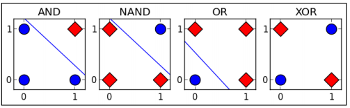
注：在吴恩达老师讲的【机器学习】课程中，最开始介绍神经网络的应用时就介绍了含有一个隐藏层的神经网络可以解决异或问题，而这是单层神经网络（也叫感知机）做不到了，当时就觉得非常神奇，之后就一直打算自己实现一下，一直到一周前才开始动手实现。自己参考【机器学习】课程中数字识别的作业题写了代码，对于作业题中给的数字图片可以达到95%左右的识别准确度。但是改成训练异或的网络时，怎么也无法得到正确的结果。后来查了一些资料才发现是因为自己有一个参数设置的有问题，而且学习率过小，迭代的次数也不够。总之，异或逻辑的实现不仅对于人工神经网络这一算法是一大突破，对于我自己对误差反向传播算法（Error Back Propagation, BP）的理解也是非常重要的过程，因此记录于此。

什么是异或

在数字逻辑中，异或是对两个运算元的一种逻辑分析类型，符号为XOR或EOR或⊕。与一般的或（OR）不同，当两两数值相同时为否，而数值不同时为真。异或的真值表如下：

XOR truth table InputOutput AB 0 0 0 0 1 1 1 0 1 1 1 0 0, false 1, true

据说在人工神经网络（artificial neural network, ANN）发展初期，由于无法实现对多层神经网络（包括异或逻辑）的训练而造成了一场ANN危机，到最后BP算法的出现，才让训练带有隐藏层的多层神经网络成为可能。因此异或的实现在ANN的发展史是也是具有里程碑意义的。异或之所以重要，是因为它相对于其他逻辑关系，例如与（AND）, 或（OR）等，异或是线性不可分的。如下图：

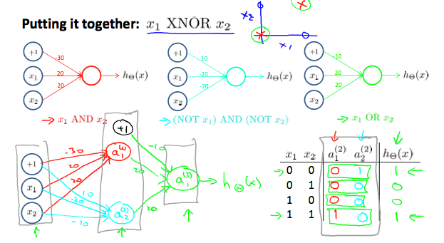
在实际应用中，异或门（Exclusive-OR gate, XOR gate）是数字逻辑中实现逻辑异或的逻辑门，这一函数能实现模为2的加法。因此，异或门可以实现计算机中的二进制加法。

异或的神经网络结构

在【机器学习】课程中，使用了AND（与），NOR（或非）和OR（或）的组合实现了XNOR（同或），与我们要实现的异或（XOR）正好相反。因此还是可以采用课程中的神经网络结构，如下图：

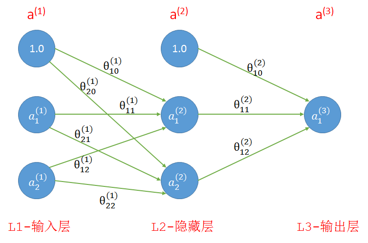
如果算上输入层我们的网络共有三层，如下图所示，其中第1层和第2层中的1分别是这两层的偏置单元。连线上是连接前后层的参数。

输入：我们一共有四个训练样本，每个样本有两个特征，分别是(0, 0), (1, 0), (0, 1), (1, 1); 理想输出：参考上面的真值表，样本中两个特征相同时为0，相异为1 参数：随机初始化，范围为(-1, 1) 关于神经网络的基础知识以及前向传播、反向传播的实现请参考下面两篇文章，写的非常精彩：

机器学习公开课笔记(4)：神经网络(Neural Network)——表示

机器学习公开课笔记(5)：神经网络(Neural Network)——学习

代码原生态的代码：

下面的实现是完全根据自己的理解和对【机器学习】课程中作业题的模仿而写成的，虽然代码质量不是非常高，但是算法的所有细节都展示出来了。

在66, 69, 70行的注释是我之前没有得到正确结果的三个原因，其中epsilon确定的是随机初始化参数的范围，例如epsilon=1，参数范围就是(-1, 1)

1 # -*- coding: utf-8 -*- 2 """ 3 Created on Tue Apr 4 10:47:51 2017 4 5 @author: xin 6 """ 7 # Neural Network for XOR 8 import numpy as np 9 import matplotlib.pyplot as plt 10 11 HIDDEN_LAYER_SIZE = 2 12 INPUT_LAYER = 2 # input feature 13 NUM_LABELS = 1 # output class number 14 X = np.array([[0, 0], [0, 1], [1, 0], [1, 1]]) 15 y = np.array([[0], [1], [1], [0]]) 16 17 18 def rand_initialize_weights(L_in, L_out, epsilon): 19 """ 20 Randomly initialize the weights of a layer with L_in 21 incoming connections and L_out outgoing connections; 22 23 Note that W should be set to a matrix of size(L_out, 1 + L_in) as 24 the first column of W handles the "bias" terms 25 """ 26 epsilon_init = epsilon 27 W = np.random.rand(L_out, 1 + L_in) * 2 * epsilon_init - epsilon_init 28 return W 29 30 31 def sigmoid(x): 32 return 1.0 / (1.0 + np.exp(-x)) 33 34 35 def sigmoid_gradient(z): 36 g = np.multiply(sigmoid(z), (1 - sigmoid(z))) 37 return g 38 39 40 def nn_cost_function(theta1, theta2, X, y): 41 m = X.shape[0] # m=4 42 # 计算所有参数的偏导数（梯度） 43 D_1 = np.zeros(theta1.shape) # Δ_1 44 D_2 = np.zeros(theta2.shape) # Δ_2 45 h_total = np.zeros((m, 1)) # 所有样本的预测值, m*1, probability 46 for t in range(m): 47 a_1 = np.vstack((np.array([[1]]), X[t:t + 1, :].T)) # 列向量, 3*1 48 z_2 = np.dot(theta1, a_1) # 2*1 49 a_2 = np.vstack((np.array([[1]]), sigmoid(z_2))) # 3*1 50 z_3 = np.dot(theta2, a_2) # 1*1 51 a_3 = sigmoid(z_3) 52 h = a_3 # 预测值h就等于a_3, 1*1 53 h_total[t,0] = h 54 delta_3 = h - y[t:t + 1, :].T # 最后一层每一个单元的误差, δ_3, 1*1 55 delta_2 = np.multiply(np.dot(theta2[:, 1:].T, delta_3), sigmoid_gradient(z_2)) # 第二层每一个单元的误差（不包括偏置单元）, δ_2, 2*1 56 D_2 = D_2 + np.dot(delta_3, a_2.T) # 第二层所有参数的误差, 1*3 57 D_1 = D_1 + np.dot(delta_2, a_1.T) # 第一层所有参数的误差, 2*3 58 theta1_grad = (1.0 / m) * D_1 # 第一层参数的偏导数，取所有样本中参数的均值，没有加正则项 59 theta2_grad = (1.0 / m) * D_2 60 J = (1.0 / m) * np.sum(-y * np.log(h_total) - (np.array([[1]]) - y) * np.log(1 - h_total)) 61 return {'theta1_grad': theta1_grad, 62 'theta2_grad': theta2_grad, 63 'J': J, 'h': h_total} 64 65 66 theta1 = rand_initialize_weights(INPUT_LAYER, HIDDEN_LAYER_SIZE, epsilon=1) # 之前的问题之一，epsilon的值设置的太小 67 theta2 = rand_initialize_weights(HIDDEN_LAYER_SIZE, NUM_LABELS, epsilon=1) 68 69 iter_times = 10000 # 之前的问题之二，迭代次数太少 70 alpha = 0.5 # 之前的问题之三，学习率太小 71 result = {'J': [], 'h': []} 72 theta_s = {} 73 for i in range(iter_times): 74 cost_fun_result = nn_cost_function(theta1=theta1, theta2=theta2, X=X, y=y) 75 theta1_g = cost_fun_result.get('theta1_grad') 76 theta2_g = cost_fun_result.get('theta2_grad') 77 J = cost_fun_result.get('J') 78 h_current = cost_fun_result.get('h') 79 theta1 -= alpha * theta1_g 80 theta2 -= alpha * theta2_g 81 result['J'].append(J) 82 result['h'].append(h_current) 83 # print(i, J, h_current) 84 if i==0 or i==(iter_times-1): 85 print('theta1', theta1) 86 print('theta2', theta2) 87 theta_s['theta1_'+str(i)] = theta1.copy() 88 theta_s['theta2_'+str(i)] = theta2.copy() 89 90 plt.plot(result.get('J')) 91 plt.show() 92 print(theta_s) 93 print(result.get('h')[0], result.get('h')[-1])

下面是输出结果：

# 随机初始化得到的参数('theta1', array([[ 0.18589823, -0.77059558, 0.62571502], [-0.79844165, 0.56069914, 0.21090703]])) ('theta2', array([[ 0.1327994 , 0.59513332, 0.34334931]]))

# 训练后得到的参数 ('theta1', array([[-3.90903729, -7.44497437, 7.20130773], [-3.76429211, 6.93482723, -7.21857912]])) ('theta2', array([[ -6.5739346 , 13.33011993, 13.3891608 ]]))

# 同上，第一次迭代和最后一次迭代得到的参数 {'theta1_0': array([[ 0.18589823, -0.77059558, 0.62571502], [-0.79844165, 0.56069914, 0.21090703]]), 'theta2_9999': array([[ -6.5739346 , 13.33011993, 13.3891608 ]]), 'theta1_9999': array([[-3.90903729, -7.44497437, 7.20130773], [-3.76429211, 6.93482723, -7.21857912]]), 'theta2_0': array([[ 0.1327994 , 0.59513332, 0.34334931]])} # 预测值h: 第1个array里是初始参数预测出来的值，第2个array中是最后一次得到的参数预测出来的值(array([[ 0.66576877], [ 0.69036552], [ 0.64994307], [ 0.67666546]]), array([[ 0.00245224], [ 0.99812746], [ 0.99812229], [ 0.00215507]]))

下面是随着迭代次数的增加，代价函数值J(θ)的变化情况：

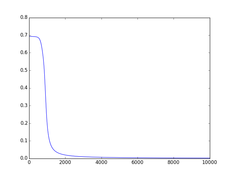
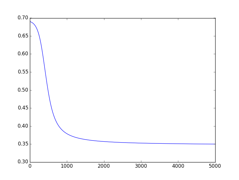
更加精炼的代码

下面这段代码是我在排除之前自己的代码中的问题时，在Stack Overflow上发现的，发帖的人也碰到了同样的问题，但原因不一样。他的代码里有一点小问题，已经修正。这段代码，相对于我自己的原生态代码，有了非常大的改进，没有限定层数和每层的单元数，代码本身也比较简洁。

说明：由于第44行，传的参数是该层的a值，而不是z值，所以第11行需要做出一点修改，其实直接传递a值是一种更方便的做法。

1 # -*- coding: utf-8 -*- 2 3 import numpy as np 4 import matplotlib.pyplot as plt 5 6 7 def sigmoid(x): 8 return 1/(1+np.exp(-x)) 9 10 def s_prime(z): 11 return np.multiply(z, 1.0-z) # 修改的地方 12 13 def init_weights(layers, epsilon): 14 weights = [] 15 for i in range(len(layers)-1): 16 w = np.random.rand(layers[i+1], layers[i]+1) 17 w = w * 2*epsilon - epsilon 18 weights.append(np.mat(w)) 19 return weights 20 21 def fit(X, Y, w): 22 # now each para has a grad equals to 0 23 w_grad = ([np.mat(np.zeros(np.shape(w[i]))) 24 for i in range(len(w))]) # len(w) equals the layer number 25 m, n = X.shape 26 h_total = np.zeros((m, 1)) # 所有样本的预测值, m*1, probability 27 for i in range(m): 28 x = X[i] 29 y = Y[0,i] 30 # forward propagate 31 a = x 32 a_s = [] 33 for j in range(len(w)): 34 a = np.mat(np.append(1, a)).T 35 a_s.append(a) # 这里保存了前L-1层的a值 36 z = w[j] * a 37 a = sigmoid(z) 38 h_total[i, 0] = a 39 # back propagate 40 delta = a - y.T 41 w_grad[-1] += delta * a_s[-1].T # L-1层的梯度 42 # 倒过来，从倒数第二层开始到第二层结束，不包括第一层和最后一层 43 for j in reversed(range(1, len(w))): 44 delta = np.multiply(w[j].T*delta, s_prime(a_s[j])) # 这里传递的参数是a，而不是z 45 w_grad[j-1] += (delta[1:] * a_s[j-1].T) 46 w_grad = [w_grad[i]/m for i in range(len(w))] 47 J = (1.0 / m) * np.sum(-Y * np.log(h_total) - (np.array([[1]]) - Y) * np.log(1 - h_total)) 48 return {'w_grad': w_grad, 'J': J, 'h': h_total} 49 50 51 X = np.mat([[0,0], 52 [0,1], 53 [1,0], 54 [1,1]]) 55 Y = np.mat([0,1,1,0]) 56 layers = [2,2,1] 57 epochs = 5000 58 alpha = 0.5 59 w = init_weights(layers, 1) 60 result = {'J': [], 'h': []} 61 w_s = {} 62 for i in range(epochs): 63 fit_result = fit(X, Y, w) 64 w_grad = fit_result.get('w_grad') 65 J = fit_result.get('J') 66 h_current = fit_result.get('h') 67 result['J'].append(J) 68 result['h'].append(h_current) 69 for j in range(len(w)): 70 w[j] -= alpha * w_grad[j] 71 if i == 0 or i == (epochs - 1): 72 # print('w_grad', w_grad) 73 w_s['w_' + str(i)] = w_grad[:] 74 75 76 plt.plot(result.get('J')) 77 plt.show() 78 print(w_s) 79 print(result.get('h')[0], result.get('h')[-1])

下面是输出的结果：

# 第一次迭代和最后一次迭代得到的参数 {'w_4999': [matrix([[ 1.51654104e-04, -2.30291680e-04, 6.20083292e-04], [ 9.15463982e-05, -1.51402782e-04, -6.12464354e-04]]), matrix([[ 0.0004279 , -0.00051928, -0.00042735]])], 'w_0': [matrix([[ 0.00172196, 0.0010952 , 0.00132499], [-0.00489422, -0.00489643, -0.00571827]]), matrix([[-0.02787502, -0.01265985, -0.02327431]])]} # 预测值h: 第1个array里是初始参数预测出来的值，第2个array中是最后一次得到的参数预测出来的值 (array([[ 0.45311095], [ 0.45519066], [ 0.4921871 ], [ 0.48801121]]), array([[ 0.00447994], [ 0.49899856], [ 0.99677373], [ 0.50145936]]))

观察上面的结果，最后一次迭代得到的结果并不是我们期待的结果，也就是第1、4个值接近于0, 第2、3个值接近于1。下面是代价函数值J(θ)随着迭代次数增加的变化情况：

从上图可以看到，J(θ)的值从2000以后就一直停留在0.35左右，因此整个网络有可能收敛到了一个局部最优解，也有可能是迭代次数不够导致的。

将迭代次数改成10000后，即epochs = 10000，基本上都是可以得到预期的结果的。其实在迭代次数少的情况下，也有可能得到预期的结果，这应该主要取决于初始的参数。

经验小结

通过阅读别人的代码确实是提高自己编程能力的一种重要方法。例如通过比较自己的原生态版代码和其他人写的代码，就可以找出自己的不足之处。其中最大的收获是：数据结构对于代码的结构和逻辑都非常重要。比如我自己写的时候，每一层是分开的，但后面的代码中将整个网络一起初始化并保存在一个list中，这就提高了代码的可扩展能力，也使得代码更加简洁！

此外，要准确的理解各种算法的细节，最好的方式就是自己实现一次。

参考文献

https://zh.wikipedia.org/wiki/%E9%80%BB%E8%BE%91%E5%BC%82%E6%88%96

https://zh.wikipedia.org/wiki/%E5%BC%82%E6%88%96%E9%97%A8

https://muxuezi.github.io/posts/10-from-the-perceptron-to-artificial-neural-networks.html

http://stackoverflow.com/q/36369335/2803344

Coursera, Andrew Ng 公开课第四周，第五周

【本文地址】

公司简介

联系我们