VGG19

2023-08-11 16:59| 来源: 网络整理| 查看: 265

先导入包

import tensorflow as tf import IPython.display as display import matplotlib.pyplot as plt import numpy as np import PIL.Image import time import functools

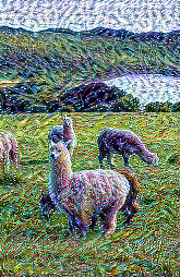
迭代了50次（次数过少）的效果

迭代800次

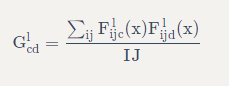
定义一个加载图像的函数，并将其最大尺寸限制为 512 像素。

创建一个简单的函数来显示图像

def tensor_to_image(tensor): tensor = tensor*255 tensor = np.array(tensor, dtype=np.uint8) if np.ndim(tensor)>3: assert tensor.shape[0] == 1 tensor = tensor[0] return PIL.Image.fromarray(tensor) def load_img(path_to_img): max_dim = 512 img = tf.io.read_file(path_to_img) img = tf.image.decode_image(img, channels=3) img = tf.image.convert_image_dtype(img, tf.float32) shape = tf.cast(tf.shape(img)[:-1], tf.float32) long_dim = max(shape) scale = max_dim / long_dim new_shape = tf.cast(shape * scale, tf.int32) img = tf.image.resize(img, new_shape) img = img[tf.newaxis, :] return img def imshow(image, title=None): if len(image.shape) > 3: image = tf.squeeze(image, axis=0) plt.imshow(image) if title: plt.title(title) content_image = load_img('1.jpg') style_image = load_img('2.jpg') plt.subplot(1, 2, 1) imshow(content_image, 'Content Image') plt.subplot(1, 2, 2) imshow(style_image, 'Style Image')

使用模型的中间层来获取图像的内容和风格表示。

从网络的输入层开始，前几个层的激励响应表示边缘和纹理等低级 feature (特征)。

随着层数加深，最后几层代表更高级的 feature (特征)——实体的部分，如轮子或眼睛。

我们使用的是 VGG19 网络结构，这是一个已经预训练好的图像分类网络。

这些中间层是从图像中定义内容和风格的表示所必需的。

对于一个输入图像，我们尝试匹配这些中间层的相应风格和内容目标的表示。

x = tf.keras.applications.vgg19.preprocess_input(content_image*255) x = tf.image.resize(x, (224, 224)) vgg = tf.keras.applications.VGG19(include_top=True, weights='imagenet') prediction_probabilities = vgg(x) prediction_probabilities.shape predicted_top_5 = tf.keras.applications.vgg19.decode_predictions(prediction_probabilities.numpy())[0] [(class_name, prob) for (number, class_name, prob) in predicted_top_5] # 现在，加载没有分类部分的 VGG19 ，并列出各层的名称： vgg = tf.keras.applications.VGG19(include_top=False, weights='imagenet') print() for layer in vgg.layers: print(layer.name) ------------------------------ input_2 block1_conv1 block1_conv2 block1_pool block2_conv1 block2_conv2 block2_pool block3_conv1 block3_conv2 block3_conv3 block3_conv4 block3_pool block4_conv1 block4_conv2 block4_conv3 block4_conv4 block4_pool block5_conv1 block5_conv2 block5_conv3 block5_conv4 block5_pool

从网络中选择中间层的输出以表示图像的风格和内容：

# 内容层将提取出我们的 feature maps （特征图） content_layers = ['block5_conv2'] # 我们感兴趣的风格层 style_layers = ['block1_conv1', 'block2_conv1', 'block3_conv1', 'block4_conv1', 'block5_conv1'] num_content_layers = len(content_layers) num_style_layers = len(style_layers)

用于表示风格和内容的中间层

那么,为什么我们预训练的图像分类网络中的这些中间层的输出允许我们定义风格和内容的表示？

从高层理解，为了使网络能够实现图像分类（该网络已被训练过），它必须理解图像。

这需要将原始图像作为输入像素并构建内部表示，这个内部表示将原始图像像素转换为对图像中存在的 feature (特征)的复杂理解。

这也是卷积神经网络能够很好地推广的一个原因：它们能够捕获不变性并定义类别（例如猫与狗）之间的 feature (特征)，这些 feature (特征)与背景噪声和其他干扰无关。

因此，将原始图像传递到模型输入和分类标签输出之间的某处的这一过程，可以视作复杂的 feature (特征)提取器。通过这些模型的中间层，我们就可以描述输入图像的内容和风格。

建立模型

使用tf.keras.applications中的网络可以让我们非常方便的利用 Keras 的功能接口提取中间层的值。

在使用功能接口定义模型时，我们需要指定输入和输出：

model = Model(inputs, outputs)

以下函数构建了一个 VGG19 模型，该模型返回一个中间层输出的列表：

def vgg_layers(layer_names): """ Creates a vgg model that returns a list of intermediate output values.""" # 加载我们的模型。加载已经在 imagenet 数据上预训练的 VGG vgg = tf.keras.applications.VGG19(include_top=False, weights='imagenet') vgg.trainable = False outputs = [vgg.get_layer(name).output for name in layer_names] model = tf.keras.Model([vgg.input], outputs) return model

然后建立模型

style_extractor = vgg_layers(style_layers) style_outputs = style_extractor(style_image*255) #查看每层输出的统计信息 for name, output in zip(style_layers, style_outputs): print(name) print(" shape: ", output.numpy().shape) print(" min: ", output.numpy().min()) print(" max: ", output.numpy().max()) print(" mean: ", output.numpy().mean()) print() ------------------------ block1_conv1 shape: (1, 336, 512, 64) min: 0.0 max: 835.5256 mean: 33.97525 block2_conv1 shape: (1, 168, 256, 128) min: 0.0 max: 4625.8857 mean: 199.82687 block3_conv1 shape: (1, 84, 128, 256) min: 0.0 max: 8789.239 mean: 230.78099 block4_conv1 shape: (1, 42, 64, 512) min: 0.0 max: 21566.135 mean: 791.24005 block5_conv1 shape: (1, 21, 32, 512) min: 0.0 max: 3189.2542 mean: 59.179478 风格计算

图像的内容由中间 feature maps (特征图)的值表示。

事实证明，图像的风格可以通过不同 feature maps (特征图)上的平均值和相关性来描述。

通过在每个位置计算 feature (特征)向量的外积，并在所有位置对该外积进行平均,可以计算出包含此信息的 Gram 矩阵。

对于特定层的 Gram 矩阵，具体计算方法如下所示：

这可以使用tf.linalg.einsum函数来实现：

def gram_matrix(input_tensor): result = tf.linalg.einsum('bijc,bijd->bcd', input_tensor, input_tensor) input_shape = tf.shape(input_tensor) num_locations = tf.cast(input_shape[1]*input_shape[2], tf.float32) return result/(num_locations)

提取风格和内容

构建一个返回风格和内容张量的模型。

class StyleContentModel(tf.keras.models.Model): def __init__(self, style_layers, content_layers): super(StyleContentModel, self).__init__() self.vgg = vgg_layers(style_layers + content_layers) self.style_layers = style_layers self.content_layers = content_layers self.num_style_layers = len(style_layers) self.vgg.trainable = False def call(self, inputs): "Expects float input in [0,1]" inputs = inputs*255.0 preprocessed_input = tf.keras.applications.vgg19.preprocess_input(inputs) outputs = self.vgg(preprocessed_input) style_outputs, content_outputs = (outputs[:self.num_style_layers], outputs[self.num_style_layers:]) style_outputs = [gram_matrix(style_output) for style_output in style_outputs] content_dict = {content_name:value for content_name, value in zip(self.content_layers, content_outputs)} style_dict = {style_name:value for style_name, value in zip(self.style_layers, style_outputs)} return {'content':content_dict, 'style':style_dict}

在图像上调用此模型，可以返回 style_layers 的 gram 矩阵（风格）和 content_layers 的内容：

extractor = StyleContentModel(style_layers, content_layers) results = extractor(tf.constant(content_image)) style_results = results['style'] print('Styles:') for name, output in sorted(results['style'].items()): print(" ", name) print(" shape: ", output.numpy().shape) print(" min: ", output.numpy().min()) print(" max: ", output.numpy().max()) print(" mean: ", output.numpy().mean()) print() print("Contents:") for name, output in sorted(results['content'].items()): print(" ", name) print(" shape: ", output.numpy().shape) print(" min: ", output.numpy().min()) print(" max: ", output.numpy().max()) print(" mean: ", output.numpy().mean()) ---------------------------------- Styles: block1_conv1 shape: (1, 64, 64) min: 0.0055228462 max: 28014.562 mean: 263.79025 block2_conv1 shape: (1, 128, 128) min: 0.0 max: 61479.49 mean: 9100.949 block3_conv1 shape: (1, 256, 256) min: 0.0 max: 545623.44 mean: 7660.976 block4_conv1 shape: (1, 512, 512) min: 0.0 max: 4320502.0 mean: 134288.84 block5_conv1 shape: (1, 512, 512) min: 0.0 max: 110005.34 mean: 1487.0381 Contents: block5_conv2 shape: (1, 26, 32, 512) min: 0.0 max: 2410.8796 mean: 13.764149 梯度下降

使用此风格和内容提取器，我们现在可以实现风格传输算法。我们通过计算每个图像的输出和目标的均方误差来做到这一点，然后取这些损失值的加权和。

设置风格和内容的目标值：

style_targets = extractor(style_image)['style'] content_targets = extractor(content_image)['content']

定义一个 tf.Variable 来表示要优化的图像。为了快速实现这一点，使用内容图像对其进行初始化（ tf.Variable 必须与内容图像的形状相同）

image = tf.Variable(content_image)

由于这是一个浮点图像，因此我们定义一个函数来保持像素值在 0 和 1 之间：

def clip_0_1(image): return tf.clip_by_value(image, clip_value_min=0.0, clip_value_max=1.0)

创建一个 optimizer 。本教程推荐 LBFGS，但 Adam 也可以正常工作：

opt = tf.optimizers.Adam(learning_rate=0.02, beta_1=0.99, epsilon=1e-1)

为了优化它，我们使用两个损失的加权组合来获得总损失：

style_weight=1e-2 content_weight=1e4 def style_content_loss(outputs): style_outputs = outputs['style'] content_outputs = outputs['content'] style_loss = tf.add_n([tf.reduce_mean((style_outputs[name]-style_targets[name])**2) for name in style_outputs.keys()]) style_loss *= style_weight / num_style_layers content_loss = tf.add_n([tf.reduce_mean((content_outputs[name]-content_targets[name])**2) for name in content_outputs.keys()]) content_loss *= content_weight / num_content_layers loss = style_loss + content_loss return loss

使用 tf.GradientTape 来更新图像。

@tf.function() def train_step(image): with tf.GradientTape() as tape: outputs = extractor(image) loss = style_content_loss(outputs) grad = tape.gradient(loss, image) opt.apply_gradients([(grad, image)]) image.assign(clip_0_1(image))

现在，我们运行几个步来测试一下：

train_step(image) train_step(image) train_step(image) tensor_to_image(image)

结果如下：

运行正常，我们来执行一个更长的优化：

import time start = time.time() epochs = 10 steps_per_epoch = 100 step = 0 for n in range(epochs): for m in range(steps_per_epoch): step += 1 train_step(image) print(".", end='') display.clear_output(wait=True) display.display(tensor_to_image(image)) print("Train step: {}".format(step)) end = time.time() print("Total time: {:.1f}".format(end-start))

【本文地址】

公司简介

联系我们