MATLAB机器人可视化

2023-09-16 13:03| 来源: 网络整理| 查看: 265

MATLAB机器人可视化

二民院小学生分类：建模仿真发布时间 2020.06.22阅读数 8625 评论数 1 1、前记:

可能用Robotics Toolbox建立的机器人模型与实际机器人在外观上存在天壤之别吧，直接将CAD软件（UG、SolidWorks、CATIA、Proe等）做好的3D模型导入MATLAB中是一个很好的选择。

下面记录MATLAB官网上的如何显示具有可视几何图形的机器人建模。

1）导入具有.stl文件的机器人与统一的机器人描述格式 (URDF) 文件相关联, 以描述机器人的视觉几何。每个刚体都有一个单独的视觉几何特征。importrobot函数对 URDF 文件进行解析, 得到机器人模型和视觉几何。使用show功能可视化的机器人模型显示在一个figure图框中。然后, 您可以通过单击组件来检查它们并右键单击以切换可见性来与模型进行交互。

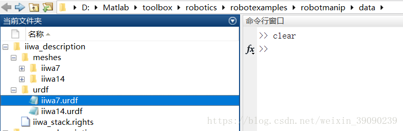
将机器人模型作为 URDF 文件导入。此 URDF 中必须正确指定.stl文件位置。要将其他.stl文件添加到单个刚性体, 请参见 addVisual .如：iiwa的URDF描述文件中的部分。

在命令窗输入代码：

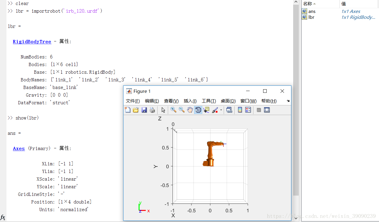
robot = importrobot('iiwa14.urdf');

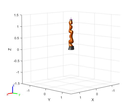
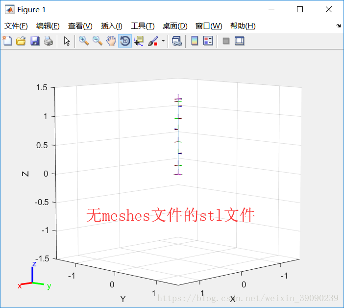
用相关的视觉模型可视化机器人。单击 "正文" 或 "框架" 进行检查。右键单击 "正文" 可切换每个可视几何图形的可见性。

代码：show(robot);%机器人显示如下

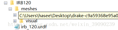
2）如此，在具有机器人的URDF文件和对应的stl文件条件下运行以上两行代码即可显示具有几何特征的可视化机器人模型。

如下：ABB机器人的IRB120

和ABB机器人的YUMI

2、仿真

机器人可视化到MATLAB环境下后，就可以做仿真了。在MATLAB的实例中可以直接学习到一些思路，代码和结果如下：

具有多个约束的轨迹规划---->

%% Plan a Reaching Trajectory With Multiple Kinematic Constraints %% Introduction % This example shows how to use generalized inverse kinematics to plan a % joint-space trajectory for a robotic manipulator. It combines multiple % constraints to generate a trajectory that guides the gripper to a cup % resting on a table. These constraints ensure that the gripper approaches % the cup in a straight line and that the gripper remains at a safe % distance from the table, without requiring the poses of the gripper to be % determined in advance. % Copyright 2016 The MathWorks, Inc. %% Set Up the Robot Model % This example uses a model of the KUKA LBR iiwa, a 7 degree-of-freedom % robot manipulator. || generates % a || model from a % description stored in a Unified Robot Description Format (URDF) file. lbr = importrobot('iiwa14.urdf'); % 14 kg payload version lbr.DataFormat = 'row'; gripper = 'iiwa_link_ee_kuka'; %% % Define dimensions for the cup. cupHeight = 0.2; cupRadius = 0.05; cupPosition = [-0.5, 0.5, cupHeight/2]; %% % Add a fixed body to the robot model representing the center of the cup. body = robotics.RigidBody('cupFrame'); setFixedTransform(body.Joint, trvec2tform(cupPosition)) addBody(lbr, body, lbr.BaseName); %% Define the Planning Problem % The goal of this example is to generate a sequence of robot % configurations that satisfy the following criteria: % % * Start in the home configuration % * No abrupt changes in robot configuration % * Keep the gripper at least 5 cm above the "table" (z = 0) % * The gripper should be aligned with the cup as it approaches % * Finish with the gripper 5 cm from the center of the cup % % This example utilizes constraint objects to generate robot configurations % that satisfy these criteria. The generated trajectory consists of five % configuration waypoints. The first waypoint, |q0|, is set as the home % configuration. Pre-allocate the rest of the configurations in % |qWaypoints| using |repmat|. numWaypoints = 5; q0 = homeConfiguration(lbr); qWaypoints = repmat(q0, numWaypoints, 1); %% % Create a || solver that accepts the following % constraint inputs: % % * Cartesian bounds - Limits the height of the gripper % * A position target - Specifies the position of the cup relative to the % gripper. % * An aiming constraint - Aligns the gripper with the cup axis % * An orientation target - Maintains a fixed orientation for the gripper % while approaching the cup % * Joint position bounds - Limits the change in joint positions between waypoints. gik = robotics.GeneralizedInverseKinematics('RigidBodyTree', lbr, ... 'ConstraintInputs', {'cartesian','position','aiming','orientation','joint'}) %% Create Constraint Objects % Create the constraint objects that are passed as inputs to the solver. % These object contain the parameters needed for each constraint. Modify % these parameters between calls to the solver as necessary. %% % Create a Cartesian bounds constraint that requires the gripper to be at % least 5 cm above the table (negative z direction). All other values are % given as |inf| or |-inf|. heightAboveTable = robotics.CartesianBounds(gripper); heightAboveTable.Bounds = [-inf, inf; ... -inf, inf; ... 0.05, inf] %% % Create a constraint on the position of the cup relative to the gripper, % with a tolerance of 5 mm. distanceFromCup = robotics.PositionTarget('cupFrame'); distanceFromCup.ReferenceBody = gripper; distanceFromCup.PositionTolerance = 0.005 %% % Create an aiming constraint that requires the z-axis of the % |iiwa_link_ee| frame to be approximately vertical, by placing the target % far above the robot. The |iiwa_link_ee| frame is oriented such that this % constraint aligns the gripper with the axis of the cup. alignWithCup = robotics.AimingConstraint('iiwa_link_ee'); alignWithCup.TargetPoint = [0, 0, 100] %% % Create a joint position bounds constraint. Set the |Bounds| property of % this constraint based on the previous configuration to limit the change % in joint positions. limitJointChange = robotics.JointPositionBounds(lbr) %% % Create an orientation constraint for the gripper with a tolerance of one % degree. This constraint requires the orientation of the gripper to match % the value specified by the |TargetOrientation| property. Use this % constraint to fix the orientation of the gripper during the final % approach to the cup. fixOrientation = robotics.OrientationTarget(gripper); fixOrientation.OrientationTolerance = deg2rad(1) %% Find a Configuration That Points at the Cup % This configuration should place the gripper at a distance from the cup, % so that the final approach can be made with the gripper properly aligned. intermediateDistance = 0.3; %% % Constraint objects have a |Weights| property which determines how the % solver treats conflicting constraints. Setting the weights of a % constraint to zero disables the constraint. For this configuration, % disable the joint position bounds and orientation constraint. limitJointChange.Weights = zeros(size(limitJointChange.Weights)); fixOrientation.Weights = 0; %% % Set the target position for the cup in the gripper frame. The cup should % lie on the z-axis of the gripper at the specified distance. distanceFromCup.TargetPosition = [0,0,intermediateDistance]; %% % Solve for the robot configuration that satisfies the input constraints % using the |gik| solver. You must specify all the input constraints. Set % that configuration as the second waypoint. [qWaypoints(2,:),solutionInfo] = gik(q0, heightAboveTable, ... distanceFromCup, alignWithCup, fixOrientation, ... limitJointChange); %% Find Configurations That Move Gripper to the Cup Along a Straight Line % Re-enable the joint position bound and orientation constraints. limitJointChange.Weights = ones(size(limitJointChange.Weights)); fixOrientation.Weights = 1; %% % Disable the align-with-cup constraint, as the orientation constraint % makes it redundant. alignWithCup.Weights = 0; %% % Set the orientation constraint to hold the orientation based on the % previous configuration (|qWaypoints(2,:)|). Get the transformation from % the gripper to the base of the robot model. Convert the homogeneous % transformation to a quaternion. fixOrientation.TargetOrientation = ... tform2quat(getTransform(lbr,qWaypoints(2,:),gripper)); %% % Define the distance between the cup and gripper for each waypoint finalDistanceFromCup = 0.05; distanceFromCupValues = linspace(intermediateDistance, finalDistanceFromCup, numWaypoints-1); %% % Define the maximum allowed change in joint positions between each % waypoint. maxJointChange = deg2rad(10); %% % Call the solver for each remaining waypoint. for k = 3:numWaypoints % Update the target position. distanceFromCup.TargetPosition(3) = distanceFromCupValues(k-1); % Restrict the joint positions to lie close to their previous values. limitJointChange.Bounds = [qWaypoints(k-1,:)' - maxJointChange, ... qWaypoints(k-1,:)' + maxJointChange]; % Solve for a configuration and add it to the waypoints array. [qWaypoints(k,:),solutionInfo] = gik(qWaypoints(k-1,:), ... heightAboveTable, ... distanceFromCup, alignWithCup, ... fixOrientation, limitJointChange); end %% Visualize the Generated Trajectory % Interpolate between the waypoints to generate a smooth trajectory. Use % || to avoid overshoots, which might % violate the joint limits of the robot. framerate = 15; r = robotics.Rate(framerate); tFinal = 10; tWaypoints = [0,linspace(tFinal/2,tFinal,size(qWaypoints,1)-1)]; numFrames = tFinal*framerate; qInterp = pchip(tWaypoints,qWaypoints',linspace(0,tFinal,numFrames))'; %% % Compute the gripper position for each interpolated configuration. gripperPosition = zeros(numFrames,3); for k = 1:numFrames gripperPosition(k,:) = tform2trvec(getTransform(lbr,qInterp(k,:), ... gripper)); end %% % Show the robot in its initial configuration along with the table and cup figure; show(lbr, qWaypoints(1,:), 'PreservePlot', false); hold on exampleHelperPlotCupAndTable(cupHeight, cupRadius, cupPosition); p = plot3(gripperPosition(1,1), gripperPosition(1,2), gripperPosition(1,3)); %% % Animate the manipulator and plot the gripper position. hold on for k = 1:size(qInterp,1) show(lbr, qInterp(k,:), 'PreservePlot', false); p.XData(k) = gripperPosition(k,1); p.YData(k) = gripperPosition(k,2); p.ZData(k) = gripperPosition(k,3); waitfor(r); end hold off %% % If you want to save the generated configurations to a MAT-file for later % use, execute the following: % % |>> save('lbr_trajectory.mat', 'tWaypoints', 'qWaypoints');| displayEndOfDemoMessage(mfilename)

3、后记

MATLAB机器人可视化的方法很多，对于URDF自己写太麻烦，可以利用SolidWorks设计出三维模型后中的插件功能直接生成。有些可以利用xml文件生成，simulink中有示例，也可查看Simscape Simscape Multibody Simulink 3D Animation Simulink Control Design 等网上资源。

如：Simscape Multibody中的一个如何将STEP文件导入的方法。

4、根据上面的solid 文件from的选项我尝试了下从Robotstudio中保存机器人各部件到MATLAB目录下然后使其可视化从Robotstudiox下保存个部件参考----->

一种从Robotstudio环境中导出机器人模型并在MATLAB下使其可视化的研究记录。结果表明还是可行的，但是运行会出现错误，需要自己定义坐标的转换关系和各部件的质量等。。。如下：

参看网址：

https://ww2.mathworks.cn/help/robotics/ref/robotics.rigidbodytree-class.html

http://www.ilovematlab.cn/thread-504445-1-1.html

https://www.zhihu.com/question/56559082/answer/150314069

https://www.zhihu.com/question/58793939/answer/343951305

https://blog.csdn.net/weixin_37719670/article/details/79027035#commentBox

https://www.zhihu.com/question/40801341/answer/134010201

https://blog.csdn.net/sunbibei/article/details/52297524

https://blog.csdn.net/weixin_39090239/article/details/80557032

https://www.youtube.com/watch?v=F2kE2vGY8_A&t=11s

https://ww2.mathworks.cn/help/physmod/sm/rigid-bodies-1.html

MATLAB

打赏 0

微信微博 QQ 图片上一篇：一知半解|MATLAB机器人建模与仿真控制（4）下一篇：MATLAB下机器人可视化与控制---simulink篇（1）

【本文地址】

公司简介

联系我们

今日新闻

推荐新闻

专题文章