| YOLOv5改进系列(三) 本文(7万字) | 您所在的位置:网站首页 › shufflenetv2参数量 › YOLOv5改进系列(三) 本文(7万字) |
YOLOv5改进系列(三) 本文(7万字)
|
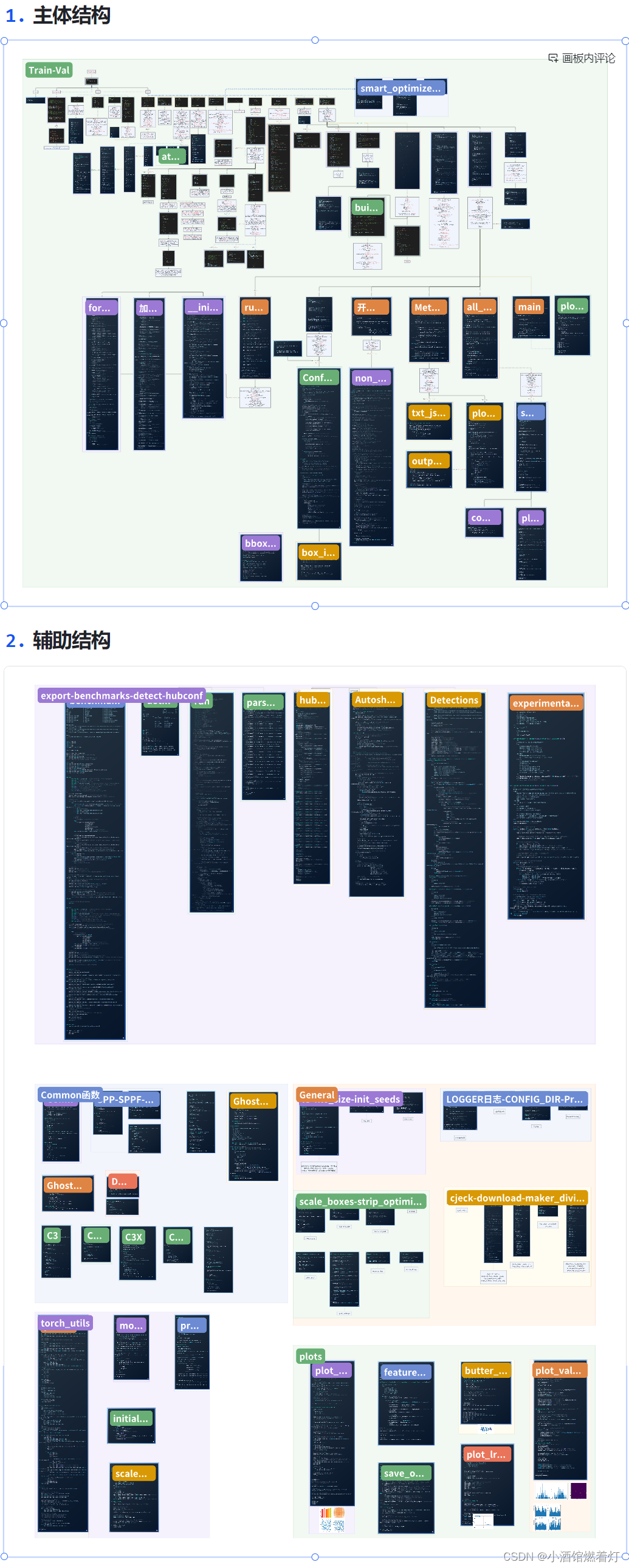
点击进入专栏: 《人工智能专栏》 Python与Python | 机器学习 | 深度学习 | 目标检测 | YOLOv5及其改进 | YOLOv8及其改进 | 关键知识点 | 各种工具教程 代码函数调用关系图(全网最详尽-重要) 因文档特殊,不能在博客正确显示,请移步以下链接! 图解YOLOv5_v7.0代码结构与调用关系(点击进入可以放大缩小等操作) 预览: MobileNetV3,是谷歌在2019年3月21日提出的轻量化网络架构,在前两个版本的基础上,加入神经网络架构搜索(NAS)和h-swish激活函数,并引入SE通道注意力机制,性能和速度都表现优异,受到学术界和工业界的追捧。 引用大佬的描述:MobileNet V3 = MobileNet v2 + SE结构 + hard-swish activation +网络结构头尾微调
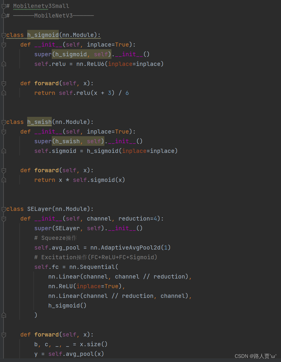
MobileNetV1&MobileNetV2&MobileNetV3总结 MobileNetV1MobileNetV2MobileNetV3标准卷积改为深度可分离卷积,降低计算量;ReLU改为ReLU6;引入Width Multiplier(α)和Resolution Multiplier(ρ),调节模型的宽度(卷积核个数)和图像分辨率;采用线性瓶颈层:将深度可分离卷积中的1×1卷积后的ReLU替换成线性激活函数;采用反向残差结构:引入Expansion layer,在进行深度分离卷积之前首先使用1×1卷积进行升维;引入Shortcut结构,在升维的1×1卷积之前与深度可分离卷积中的1×1卷积之后进行shortcut连接;采用增加了SE机制的Bottleneck模块结构;使用了一种新的激活函数h-swish(x)替代MobileNetV2中的ReLU6激活函数;网络结构搜索中,结合两种技术:资源受限的NAS(platform-aware NAS)与NetAdapt;修改了MobileNetV2网络端部最后阶段; 1.2 MobileNetV3相关技术(1)引入MobileNetV1的深度可分离卷积 (2)引入MobileNetV2的具有线性瓶颈的倒残差结构 (3)引入基于squeeze and excitation结构的轻量级注意力模型(SE) (4)使用了一种新的激活函数h-swish(x) (5)网络结构搜索中,结合两种技术:资源受限的NAS(platform-aware NAS)与NetAdapt (6)修改了MobileNetV2网络端部最后阶段 更多介绍,还是看上面的链接吧~ 二、YOLOv5结合MobileNetV3_smallMobileNetV3详细解读 MobileNetV3详解2 2.1 添加顺序之前在讲添加注意力机制时我们就介绍过改进网络的顺序,替换主干网络也是大同小异的。 (1)models/common.py --> 加入新增的网络结构 (2) models/yolo.py --> 设定网络结构的传参细节,将MobileNetV3类名加入其中。(当新的自定义模块中存在输入输出维度时,要使用qw调整输出维度) (3) models/yolov5*.yaml --> 修改现有模型结构配置文件 当引入新的层时,要修改后续的结构中的from参数当仅替换主千网络时,要注意特征图的变换,/8,/16,/32(4) train.py --> 修改‘–cfg’默认参数,训练时指定模型结构配置文件 2.2 具体添加步骤 第①步:在common.py中添加MobileNetV3模块将以下代码复制粘贴到common.py文件的末尾 # Mobilenetv3Small # ——————MobileNetV3—————— import torch import torch.nn as nn # 定义一个Hard Sigmoid函数,用于SELayer中 class h_sigmoid(nn.Module): def __init__(self, inplace=True): super(h_sigmoid, self).__init__() self.relu = nn.ReLU6(inplace=inplace) def forward(self, x): return self.relu(x + 3) / 6 # 定义一个Hard Swish函数,用于SELayer中 class h_swish(nn.Module): def __init__(self, inplace=True): super(h_swish, self).__init__() self.sigmoid = h_sigmoid(inplace=inplace) def forward(self, x): return x * self.sigmoid(x) # 定义Squeeze-and-Excitation(SE)模块 class SELayer(nn.Module): def __init__(self, channel, reduction=4): super(SELayer, self).__init__() # Squeeze操作:全局平均池化 self.avg_pool = nn.AdaptiveAvgPool2d(1) # Excitation操作(FC+ReLU+FC+Sigmoid) self.fc = nn.Sequential( nn.Linear(channel, channel // reduction), # 全连接层,将通道数降低为channel // reduction nn.ReLU(inplace=True), nn.Linear(channel // reduction, channel), # 全连接层,恢复到原始通道数 h_sigmoid() # 使用Hard Sigmoid激活函数 ) def forward(self, x): b, c, _, _ = x.size() y = self.avg_pool(x) # 对输入进行全局平均池化 y = y.view(b, c) # 将池化后的结果展平为二维张量 y = self.fc(y).view(b, c, 1, 1) # 通过全连接层计算每个通道的权重,并将其变成与输入相同的形状 return x * y # 将输入与权重相乘以实现通道注意力机制 # 定义卷积-批归一化-激活函数模块 class conv_bn_hswish(nn.Module): def __init__(self, c1, c2, stride): super(conv_bn_hswish, self).__init__() self.conv = nn.Conv2d(c1, c2, 3, stride, 1, bias=False) # 3x3卷积层 self.bn = nn.BatchNorm2d(c2) # 批归一化层 self.act = h_swish() # 使用Hard Swish激活函数 def forward(self, x): return self.act(self.bn(self.conv(x))) # 卷积 - 批归一化 - 激活函数 def fuseforward(self, x): return self.act(self.conv(x)) # 融合版本的前向传播,省略了批归一化 # 定义MobileNetV3的基本模块 class MobileNetV3(nn.Module): def __init__(self, inp, oup, hidden_dim, kernel_size, stride, use_se, use_hs): super(MobileNetV3, self).__init__() assert stride in [1, 2] # 断言,要求stride必须是1或2 self.identity = stride == 1 and inp == oup # 如果stride为1且输入通道数等于输出通道数,则为恒等映射 if inp == hidden_dim: self.conv = nn.Sequential( nn.Conv2d(hidden_dim, hidden_dim, kernel_size, stride, (kernel_size - 1) // 2, groups=hidden_dim, bias=False), # 深度可分离卷积层 nn.BatchNorm2d(hidden_dim), # 批归一化层 h_swish() if use_hs else nn.ReLU(inplace=True), # 使用Hard Swish或ReLU激活函数 SELayer(hidden_dim) if use_se else nn.Sequential(), # 使用SELayer或空的Sequential nn.Conv2d(hidden_dim, oup, 1, 1, 0, bias=False), # 1x1卷积层 nn.BatchNorm2d(oup) # 批归一化层 ) else: self.conv = nn.Sequential( nn.Conv2d(inp, hidden_dim, 1, 1, 0, bias=False), # 1x1卷积层,用于通道扩张 nn.BatchNorm2d(hidden_dim), # 批归一化层 h_swish() if use_hs else nn.ReLU(inplace=True), # 使用Hard Swish或ReLU激活函数 nn.Conv2d(hidden_dim, hidden_dim, kernel_size, stride, (kernel_size - 1) // 2, groups=hidden_dim, bias=False), # 深度可分离卷积层 nn.BatchNorm2d(hidden_dim), # 批归一化层 SELayer(hidden_dim) if use_se else nn.Sequential(), # 使用SELayer或空的Sequential h_swish() if use_hs else nn.ReLU(inplace=True), # 使用Hard Swish或ReLU激活函数 nn.Conv2d(hidden_dim, oup, 1, 1, 0, bias=False), # 1x1卷积层 nn.BatchNorm2d(oup) # 批归一化层 ) def forward(self, x): y = self.conv(x) # 通过卷积层 if self.identity: return x + y # 恒等映射 else: return y # 非恒等映射如下图所示:
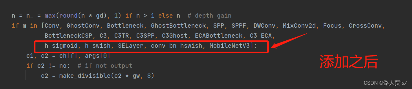
首先找到yolo.py里面parse_model函数的这一行
加入h_sigmoid,h_swish,SELayer,conv_bn_hswish,MobileNetV3五个模块
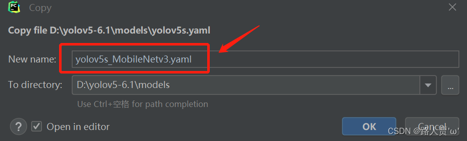
首先在models文件夹下复制yolov5s.yaml 文件,粘贴并重命名为 yolov5s_MobileNetv3.yaml
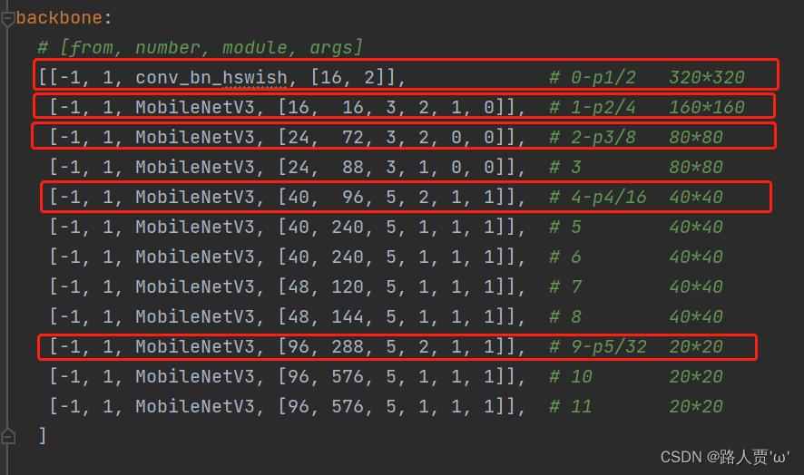
根据网络结构我们可以看出MobileNetV3模块包含六个参数[out_ch, hidden_ch, kernel_size, stride, use_se, use_hs]: out_ch: 输出通道hidden_ch: 表示在Inverted residuals中的扩张通道数kernel_size: 卷积核大小stride: 步长use_se: 表示是否使用 SELayer,使用了是1,不使用是0use_hs: 表示使用 h_swish 还是 ReLU,使用h_swish是1,使用 ReLU是0修改的时候,需要注意/8,/16,/32等位置特征图的变换
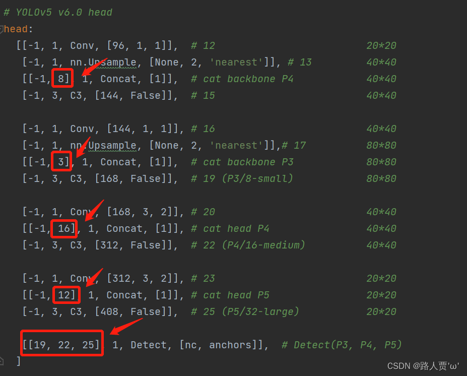
同样的,head部分这几个concat的层也要做修改:
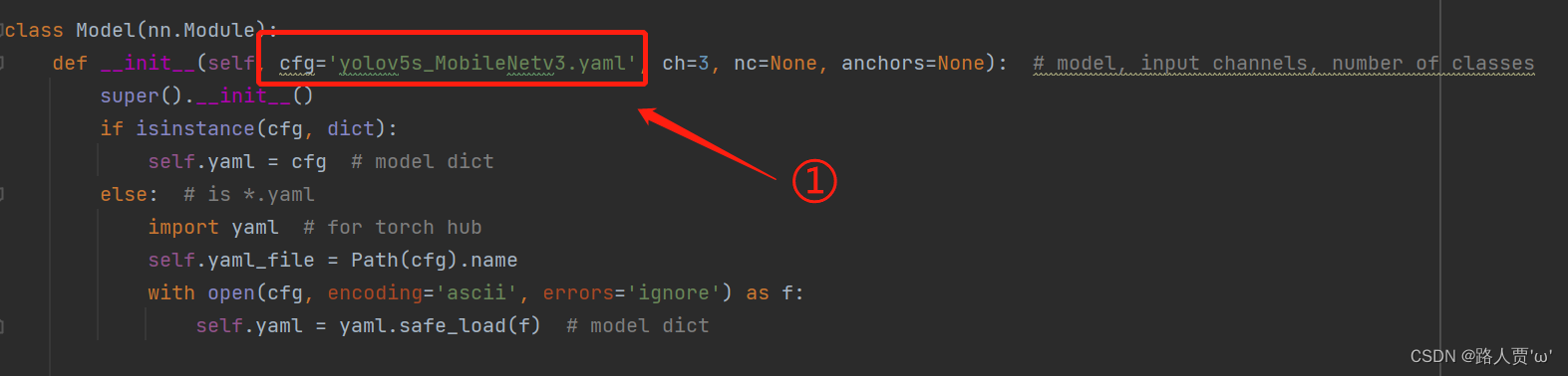
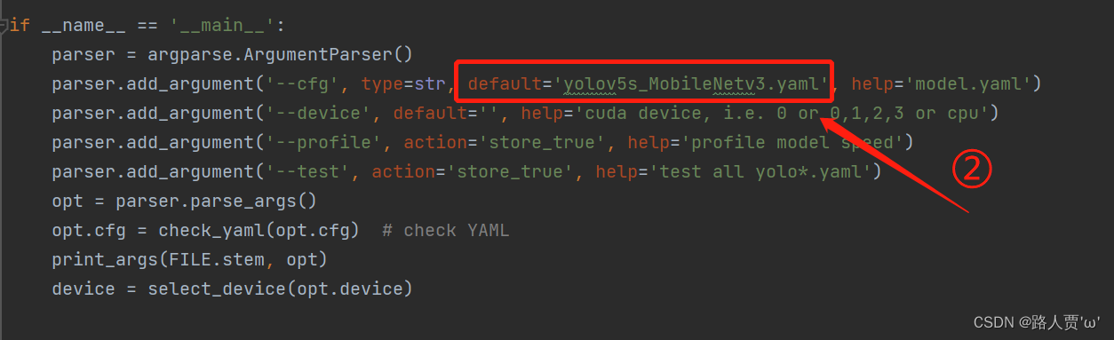
yaml文件修改后代码如下: # YOLOv5 🚀 by Ultralytics, GPL-3.0 license # Parameters nc: 80 # number of classes depth_multiple: 1.0 # model depth multiple width_multiple: 1.0 # layer channel multiple anchors: - [10,13, 16,30, 33,23] # P3/8 - [30,61, 62,45, 59,119] # P4/16 - [116,90, 156,198, 373,326] # P5/32 # Mobilenetv3-small backbone # MobileNetV3_InvertedResidual [out_ch, hid_ch, k_s, stride, SE, HardSwish] backbone: # [from, number, module, args] [[-1, 1, conv_bn_hswish, [16, 2]], # 0-p1/2 320*320 [-1, 1, MobileNetV3, [16, 16, 3, 2, 1, 0]], # 1-p2/4 160*160 [-1, 1, MobileNetV3, [24, 72, 3, 2, 0, 0]], # 2-p3/8 80*80 [-1, 1, MobileNetV3, [24, 88, 3, 1, 0, 0]], # 3 80*80 [-1, 1, MobileNetV3, [40, 96, 5, 2, 1, 1]], # 4-p4/16 40*40 [-1, 1, MobileNetV3, [40, 240, 5, 1, 1, 1]], # 5 40*40 [-1, 1, MobileNetV3, [40, 240, 5, 1, 1, 1]], # 6 40*40 [-1, 1, MobileNetV3, [48, 120, 5, 1, 1, 1]], # 7 40*40 [-1, 1, MobileNetV3, [48, 144, 5, 1, 1, 1]], # 8 40*40 [-1, 1, MobileNetV3, [96, 288, 5, 2, 1, 1]], # 9-p5/32 20*20 [-1, 1, MobileNetV3, [96, 576, 5, 1, 1, 1]], # 10 20*20 [-1, 1, MobileNetV3, [96, 576, 5, 1, 1, 1]], # 11 20*20 ] # YOLOv5 v6.0 head head: [[-1, 1, Conv, [96, 1, 1]], # 12 20*20 [-1, 1, nn.Upsample, [None, 2, 'nearest']], # 13 40*40 [[-1, 8], 1, Concat, [1]], # cat backbone P4 40*40 [-1, 3, C3, [144, False]], # 15 40*40 [-1, 1, Conv, [144, 1, 1]], # 16 40*40 [-1, 1, nn.Upsample, [None, 2, 'nearest']],# 17 80*80 [[-1, 3], 1, Concat, [1]], # cat backbone P3 80*80 [-1, 3, C3, [168, False]], # 19 (P3/8-small) 80*80 [-1, 1, Conv, [168, 3, 2]], # 20 40*40 [[-1, 16], 1, Concat, [1]], # cat head P4 40*40 [-1, 3, C3, [312, False]], # 22 (P4/16-medium) 40*40 [-1, 1, Conv, [312, 3, 2]], # 23 20*20 [[-1, 12], 1, Concat, [1]], # cat head P5 20*20 [-1, 3, C3, [408, False]], # 25 (P5/32-large) 20*20 [[19, 22, 25], 1, Detect, [nc, anchors]], # Detect(P3, P4, P5) ] 第④步:验证是否加入成功在yolo.py 文件里面配置改为我们刚才自定义的yolov5s_MobileNetv3.yaml
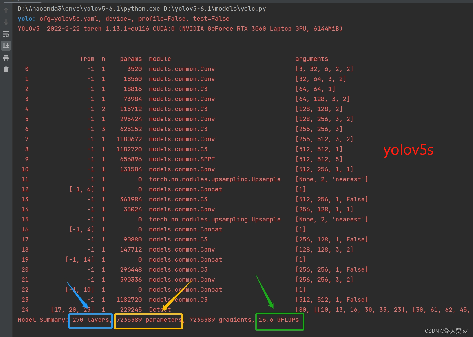
我们和原始的yolov5s.py进行对比
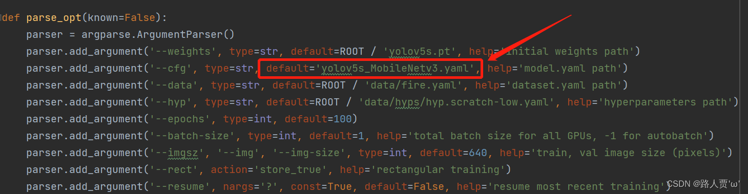
可以看到替换主干网络为MobileNetV3之后层数变多了,可以学习到更多的特征;参数量由原来的700多万减少为500多万,大幅度减少了;GFLOPs由16.6变为12.2。 第⑤步:修改train.py中 ‘–cfg’默认参数我们先找到 train.py 文件的parse_opt函数,然后将第二行**‘–cfg’的 default改为’models/yolov5s_MobileNetv3.yaml** ',然后就可以开始训练啦~
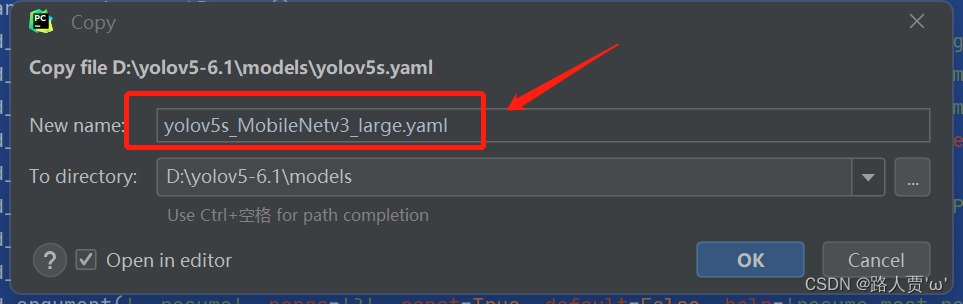
MobileNetV3_large和MobileNetV3_small区别在于yaml文件中head中concat连接不同,深度因子和宽度因子不同。 接下来我们就直接改动yaml的部分,其余参考上面步骤。 第③步:创建自定义的yaml文件同样,首先在models文件夹下复制yolov5s.yaml 文件,粘贴并重命名为 yolov5s_MobileNetv3_large.yaml
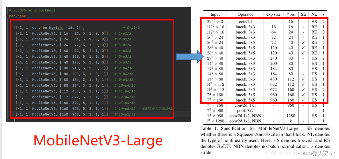
然后根据MobileNetv3的网络结构来修改配置文件。
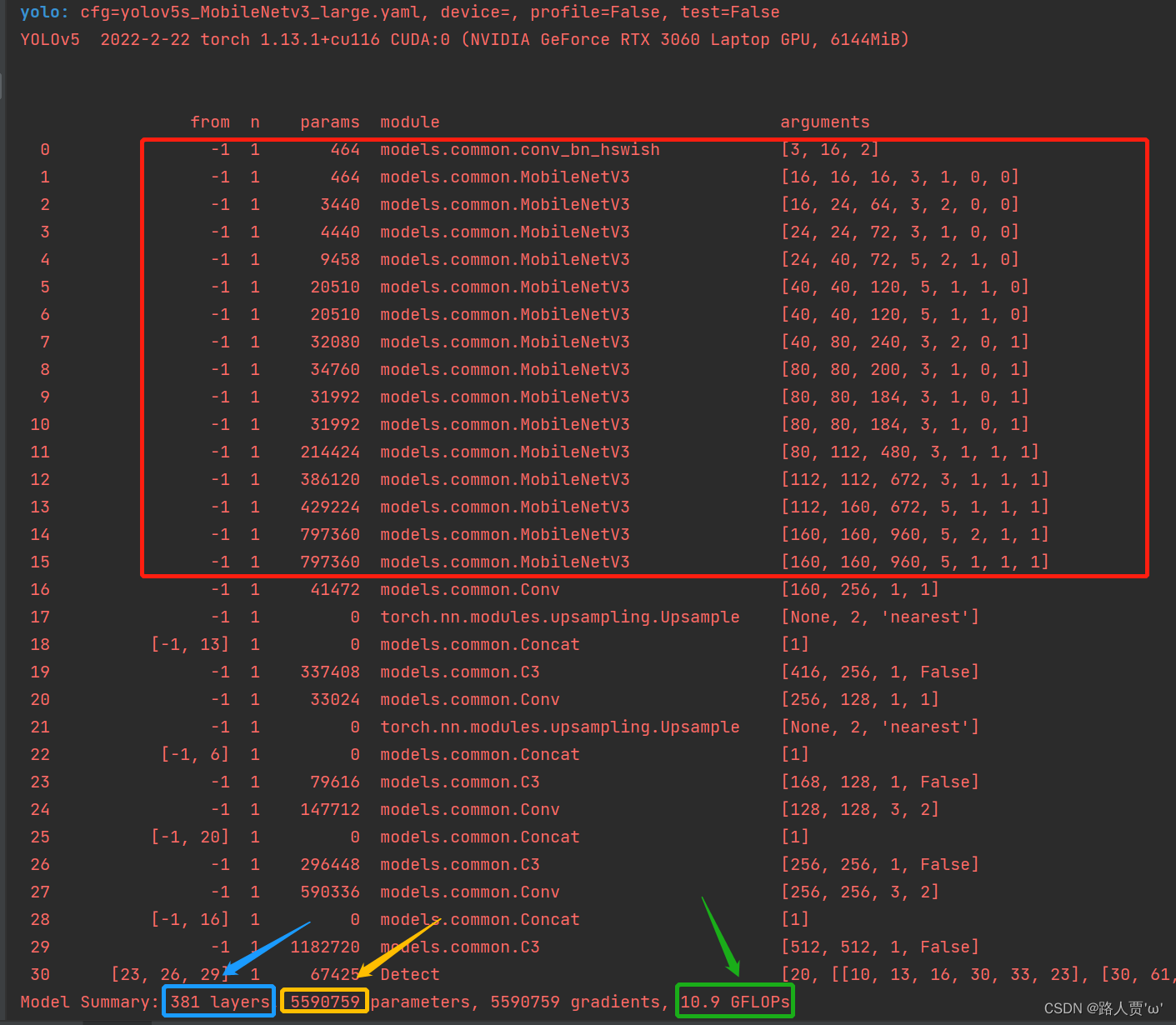
修改后代码如下: # Parameters nc: 20 # number of classes depth_multiple: 1.0 # model depth multiple width_multiple: 1.0 # layer channel multiple anchors: - [10,13, 16,30, 33,23] # P3/8 - [30,61, 62,45, 59,119] # P4/16 - [116,90, 156,198, 373,326] # P5/32 # YOLOv5 v6.0 backbone backbone: [[-1, 1, conv_bn_hswish, [16, 2]], # 0-p1/2 [-1, 1, MobileNetV3, [ 16, 16, 3, 1, 0, 0]], # 1-p1/2 [-1, 1, MobileNetV3, [ 24, 64, 3, 2, 0, 0]], # 2-p2/4 [-1, 1, MobileNetV3, [ 24, 72, 3, 1, 0, 0]], # 3-p2/4 [-1, 1, MobileNetV3, [ 40, 72, 5, 2, 1, 0]], # 4-p3/8 [-1, 1, MobileNetV3, [ 40, 120, 5, 1, 1, 0]], # 5-p3/8 [-1, 1, MobileNetV3, [ 40, 120, 5, 1, 1, 0]], # 6-p3/8 [-1, 1, MobileNetV3, [ 80, 240, 3, 2, 0, 1]], # 7-p4/16 [-1, 1, MobileNetV3, [ 80, 200, 3, 1, 0, 1]], # 8-p4/16 [-1, 1, MobileNetV3, [ 80, 184, 3, 1, 0, 1]], # 9-p4/16 [-1, 1, MobileNetV3, [ 80, 184, 3, 1, 0, 1]], # 10-p4/16 [-1, 1, MobileNetV3, [112, 480, 3, 1, 1, 1]], # 11-p4/16 [-1, 1, MobileNetV3, [112, 672, 3, 1, 1, 1]], # 12-p4/16 [-1, 1, MobileNetV3, [160, 672, 5, 1, 1, 1]], # 13-p4/16 [-1, 1, MobileNetV3, [160, 960, 5, 2, 1, 1]], # 14-p5/32 原672改为原算法960 [-1, 1, MobileNetV3, [160, 960, 5, 1, 1, 1]], # 15-p5/32 ] # YOLOv5 v6.0 head head: [ [ -1, 1, Conv, [ 256, 1, 1 ] ], [ -1, 1, nn.Upsample, [ None, 2, 'nearest' ] ], [ [ -1, 13], 1, Concat, [ 1 ] ], # cat backbone P4 [ -1, 1, C3, [ 256, False ] ], # 13 [ -1, 1, Conv, [ 128, 1, 1 ] ], [ -1, 1, nn.Upsample, [ None, 2, 'nearest' ] ], [ [ -1, 6 ], 1, Concat, [ 1 ] ], # cat backbone P3 [ -1, 1, C3, [ 128, False ] ], # 17 (P3/8-small) [ -1, 1, Conv, [ 128, 3, 2 ] ], [ [ -1, 20 ], 1, Concat, [ 1 ] ], # cat head P4 [ -1, 1, C3, [ 256, False ] ], # 20 (P4/16-medium) [ -1, 1, Conv, [ 256, 3, 2 ] ], [ [ -1, 16 ], 1, Concat, [ 1 ] ], # cat head P5 [ -1, 1, C3, [ 512, False ] ], # 23 (P5/32-large) [ [ 23, 26, 29 ], 1, Detect, [ nc, anchors ] ], # Detect(P3, P4, P5) ]网络运行结果:
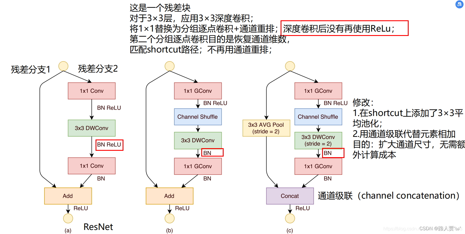
我们可以看到MobileNetV3-large模型比MobileNetV3-small多了更多的MobileNet_Block结构,残差倒置结构中通道数维度也增大了许多,速度比YOLOv5s慢将近一半,但是参数变少,效果介乎MobileNetV3-small和YOLOv5s之间,可以作为模型对比,凸显自己模型优势。 PS:如果训练之后发现掉点纯属正常现象,因为轻量化网络在提速减少计算量的同时会降低精度。 ShuffleNetV2ShuffleNetV2详细解读 ShuffleNetV2实现 一、ShuffleNet介绍ShuffleNet系列轻量级卷积神经网络由旷世提出,也是非常有趣的轻量级卷积神经网络,它提出了通道混合的概念,改善了分组卷积存在的问题,加强各组卷积之间的特征交互和信息交流,在改善模型的特征提取方式的同时,增强特征提取的全面性。 1.1 ShuffleNet V1简介 ShuffleNet V1是计算效率极高的CNN架构,该架构是专为计算能力非常有限(例如10-150 MFLOP)的移动设备设计的。新架构利用了两个新的操作,逐点组卷积和通道混洗,可以在保持准确性的同时大大降低计算成本。 ImageNet分类和MS COCO对象检测的实验证明了ShuffleNet V1优于其他结构的性能,例如在40个MFLOP的计算预算下,比最近的MobileNet [12]在ImageNet分类任务上的top-1错误要低(绝对7.8%)。在基于ARM的移动设备上,ShuffleNet V1的实际速度是AlexNet的13倍,同时保持了相当的准确性。 创新点 分组逐点卷积(pointwise group convolution)通道重排(channel shuffle)网络模型结构
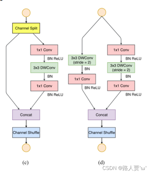
图(a)为一个Resdual block ①1×1卷积(降维)+3×3深度卷积+1×1卷积(升维)②之间有BN和ReLU③最后通过add相加图(b)为输入输出特征图大小不变的ShuffleNet Unit ①将第一个用于降低通道数的1×1卷积改为1×1分组卷积 + Channel Shuffle②去掉原3×3深度卷积后的ReLU③ 将第二个用于扩增通道数的1×1卷积改为1×1分组卷积图(c)为输出特征图大小为输入特征图大小一半的ShuffleNet Unit ①将第一个用于降低通道数的1×1卷积改为1×1分组卷积 +Channel Shuffle②令原3×3深度卷积的步长stride=2, 并且去掉深度卷积后的ReLU③将第二个用于扩增通道数的1×1卷积改为1×1分组卷积④shortcut上添加一个3×3平均池化层(stride=2)用于匹配特征图大小⑤对于块的输出,将原来的add方式改为concat方式 1.2 ShuffleNet V2简介 模型执行效率的准则不能完全取决于FLOPs,经常发现FLOPs差不多的两个模型的运算速度却不一样,因为FLOPs仅仅反映了模型的乘加次数,这种评价往往是片面的。影响模型运行速度的另一个指标也很重要,那就是MAC(memory access cost)内存访问成本。作者充分考虑了不同结构的MAC,从而设计了更加高效的网络模型ShuffleNet V2。 创新点 提出了四条实用准则: (1)使用“平衡卷积"(相等的通道数)(2)注意使用组卷积的成本(3)降低碎片化程度(4)减少逐元素操作网络模型结构
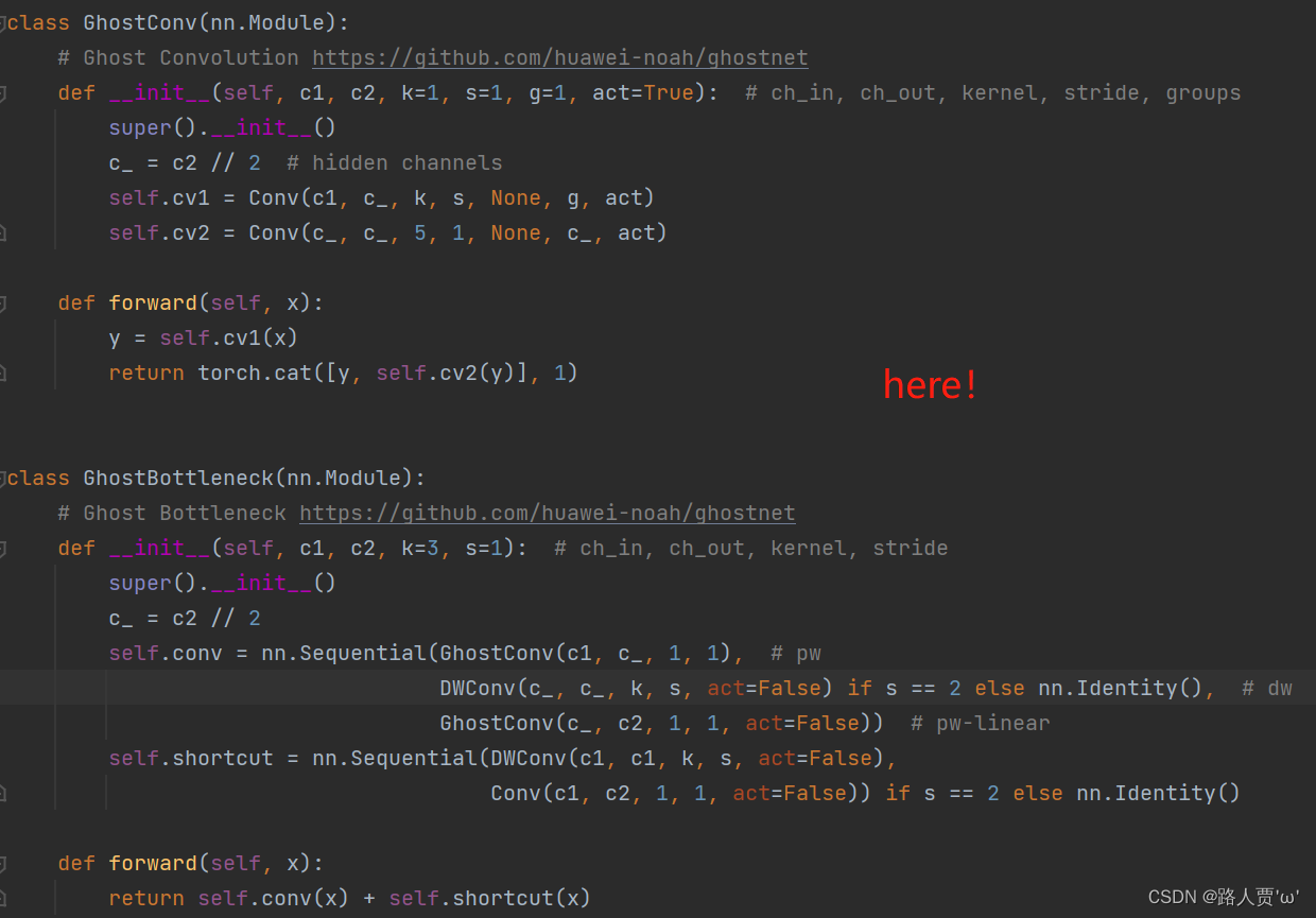
© ShuffleNet V2 的基本单元 ①增加了Channel Split操作,实际上就是把输入通道分为两个部分。②根据G1: 左边分支做恒等映射,右边的分支包含3个连续的卷积,并且输入和输出通道相同,每个分支中的卷积层的输入输出通道数都一致。③根据G2: 两个1x1卷积不再是组卷积。④根据G3: 减少基本单元数。因此有一个分支不做任何操作,直接做恒等映射。⑤根据G4: 两个分支的输出不再是Add元素,而是concat在一起,紧接着是对两个分支concat结果进行channle shuffle,以保证两个分支信息交流。(d) 用于空间下采样 (2×) 的 ShuffleNet V2 单元 对于下采样模块,不再有channel split,每个分支都有stride=2的下采样,最后concat在一起后,特征图空间大小减半,但是通道数翻倍。 二、YOLOv5结合ShuffleNet V2 2.1 添加顺序之前在讲添加注意力机制时我们就介绍过改进网络的顺序,替换主干网络也是大同小异的。 (1)models/common.py --> 加入新增的网络结构 (2) models/yolo.py --> 设定网络结构的传参细节,将ShuffleNet V2类名加入其中。(当新的自定义模块中存在输入输出维度时,要使用qw调整输出维度) (3) models/yolov5*.yaml --> 修改现有模型结构配置文件 当引入新的层时,要修改后续的结构中的from参数当仅替换主千网络时,要注意特征图的变换,/8,/16,/32(4) train.py --> 修改‘–cfg’默认参数,训练时指定模型结构配置文件 2.2 具体添加步骤 第①步:在common.py中添加ShuffleNet V2模块将以下代码复制粘贴到common.py文件的末尾 # 通道重排,跨group信息交流 import torch import torch.nn as nn # 定义通道混洗函数,用于ShuffleNet def channel_shuffle(x, groups): batchsize, num_channels, height, width = x.data.size() channels_per_group = num_channels // groups # 重塑张量形状,将通道分组并重新排列 x = x.view(batchsize, groups, channels_per_group, height, width) x = torch.transpose(x, 1, 2).contiguous() # 展平张量 x = x.view(batchsize, -1, height, width) return x # 定义CBRM模块(Convolution - BatchNormalization - ReLU - MaxPooling) class CBRM(nn.Module): def __init__(self, c1, c2): # 输入通道数c1,输出通道数c2 super(CBRM, self).__init__() self.conv = nn.Sequential( nn.Conv2d(c1, c2, kernel_size=3, stride=2, padding=1, bias=False), # 3x3卷积层 nn.BatchNorm2d(c2), # 批归一化层 nn.ReLU(inplace=True), # ReLU激活函数 ) self.maxpool = nn.MaxPool2d(kernel_size=3, stride=2, padding=1, dilation=1, ceil_mode=False) def forward(self, x): return self.maxpool(self.conv(x)) # 卷积 - 批归一化 - ReLU - 最大池化 # 定义ShuffleNet中的Shuffle Block模块 class Shuffle_Block(nn.Module): def __init__(self, ch_in, ch_out, stride): super(Shuffle_Block, self).__init__() if not (1 加入新增的网络结构(2) models/yolo.py --> 设定网络结构的传参细节,将GhostNet类名加入其中。(当新的自定义模块中存在输入输出维度时,要使用qw调整输出维度) (3) models/yolov5*.yaml --> 修改现有模型结构配置文件 当引入新的层时,要修改后续的结构中的from参数当仅替换主千网络时,要注意特征图的变换,/8,/16,/32(4) train.py --> 修改‘–cfg’默认参数,训练时指定模型结构配置文件 2.2 具体添加步骤 第①步:在common.py中添加GhostNet模块这次比较特殊,因为在最新版本的YOLOv5-6.1源码中,作者已经加入了Ghost模块,在models/common.py 文件下 (就在Focus类的下面) import torch import torch.nn as nn # Squeeze-and-Excitation (SE) 模块定义 class SeBlock(nn.Module): def __init__(self, in_channel, reduction=4): super().__init__() # Squeeze:全局平均池化层 self.Squeeze = nn.AdaptiveAvgPool2d(1) # Excitation:两层全连接层(1x1卷积) self.Excitation = nn.Sequential( nn.Conv2d(in_channel, in_channel // reduction, kernel_size=1), # 1x1卷积,通道数减少 nn.ReLU(), nn.Conv2d(in_channel // reduction, in_channel, kernel_size=1), # 1x1卷积,通道数恢复 nn.Sigmoid() # Sigmoid激活函数 ) def forward(self, x): y = self.Squeeze(x) # 对输入进行全局平均池化 output = self.Excitation(y) # 通过Excitation模块计算权重 return x * (output.expand_as(x)) # 使用权重对输入进行加权求和 # Ghost Bottleneck定义 class G_bneck(nn.Module): def __init__(self, c1, c2, midc, k=5, s=1, use_se=False): # ch_in, ch_mid, ch_out, kernel, stride, use_se super().__init__() assert s in [1, 2] c_ = midc # 中间通道数 # 构建卷积层序列 self.conv = nn.Sequential( GhostConv(c1, c_, 1, 1), # 1x1卷积,通道数减少到c_ Conv(c_, c_, 3, s=2, p=1, g=c_, act=False) if s == 2 else nn.Identity(), # dw卷积,可选stride=2 # Squeeze-and-Excite模块,如果use_se为True SeBlock(c_) if use_se else nn.Sequential(), GhostConv(c_, c2, 1, 1, act=False) # 1x1卷积,通道数恢复到c2 ) # 构建shortcut层,确保输入输出通道数和大小一致 self.shortcut = nn.Identity() if (c1 == c2 and s == 1) else \ nn.Sequential(Conv(c1, c1, 3, s=s, p=1, g=c1, act=False), Conv(c1, c2, 1, 1, act=False)) # 避免stride=2时通道数改变的情况 def forward(self, x): return self.conv(x) + self.shortcut(x) # 输出是卷积结果与shortcut相加的结果如下图所示:
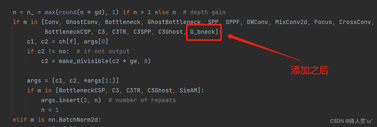
首先找到yolo.py里面parse_model函数的这一行
加入 G_bneck 这个模块
同样的,在models/hub/文件夹下,给出了yolo5s-ghost.yaml文件,因此我们直接使用即可
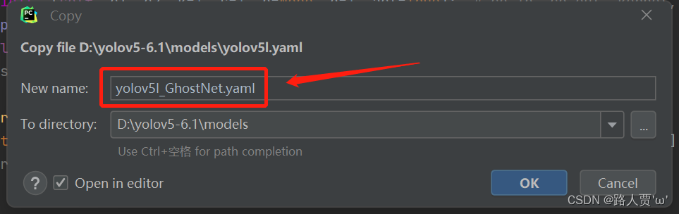
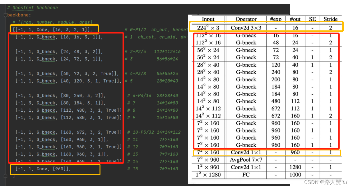
(你以为这篇文章就要这么水过去了吗✧ (≖ ‿ ≖)✧。。。 当然不可能啦!:.゚ヽ(。◕‿◕。)ノ゚.:。+゚) 参考了大佬YOLOv5/v7 更换骨干网络之 GhostNet_迪菲赫尔曼的博客-CSDN博客的代码 接下来我们说一下yolo5l_GhostNet.yaml 的写法 首先在models文件夹下复制yolov5l.yaml 文件,粘贴并重命名为 yolo5l_GhostNet.yaml
然后根据GhostNet的网络结构来修改配置文件。
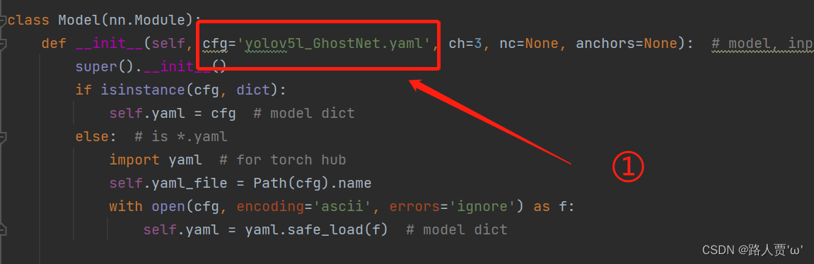
完整代码如下: # YOLOv5 🚀 by Ultralytics, GPL-3.0 license # Parameters nc: 80 # number of classes depth_multiple: 1.0 # model depth multiple width_multiple: 1.0 # layer channel multiple anchors: - [10,13, 16,30, 33,23] # P3/8 - [30,61, 62,45, 59,119] # P4/16 - [116,90, 156,198, 373,326] # P5/32 # Ghostnet backbone backbone: # [from, number, module, args] [[-1, 1, Conv, [16, 3, 2, 1]], # 0-P1/2 ch_out, kernel, stride, padding, groups 224*224*3 [-1, 1, G_bneck, [16, 16, 3, 1]], # 1 ch_out, ch_mid, dw-kernel, stride 112*112*16 [-1, 1, G_bneck, [24, 48, 3, 2]], # 2-P2/4 112*112*16 [-1, 1, G_bneck, [24, 72, 3, 1]], # 3 56*56*24 [-1, 1, G_bneck, [40, 72, 3, 2, True]], # 4-P3/8 56*56*24 [-1, 1, G_bneck, [40, 120, 3, 1, True]], # 5 28*28*40 [-1, 1, G_bneck, [80, 240, 3, 2]], # 6-P4/16 28*28*40 [-1, 3, G_bneck, [80, 184, 3, 1]], # 7 14*14*80 [-1, 1, G_bneck, [112, 480, 3, 1, True]], # 8 14*14*80 [-1, 1, G_bneck, [112, 480, 3, 1, True]], # 9 14*14*80 [-1, 1, G_bneck, [160, 672, 3, 2, True]], # 10-P5/32 14*14*112 [-1, 1, G_bneck, [160, 960, 3, 1]], # 11 7*7*160 [-1, 1, G_bneck, [160, 960, 3, 1, True]], # 12 7*7*160 [-1, 1, G_bneck, [160, 960, 3, 1]], # 13 7*7*160 [-1, 1, G_bneck, [160, 960, 3, 1, True]], # 14 7*7*160 [-1, 1, Conv, [960]], # 15 7*7*160 ] # YOLOv5 v6.0 head head: [[-1, 1, Conv, [512, 1, 1]], # 16 [-1, 1, nn.Upsample, [None, 2, 'nearest']], # 17 [[-1, 9], 1, Concat, [1]], # 18 cat backbone P4 [-1, 3, C3, [512, False]], # 19 [-1, 1, Conv, [256, 1, 1]], # 20 [-1, 1, nn.Upsample, [None, 2, 'nearest']], # 21 [[-1, 5], 1, Concat, [1]], # 22 cat backbone P3 [-1, 3, C3, [256, False]], # 23 (P3/8-small) [-1, 1, Conv, [256, 3, 2]], # 24 [[-1, 20], 1, Concat, [1]], # 25 cat head P4 [-1, 3, C3, [512, False]], # 26 (P4/16-medium) [-1, 1, Conv, [512, 3, 2]], # 27 [[-1, 15], 1, Concat, [1]], # 28 cat head P5 [-1, 3, C3, [1024, False]], # 29 (P5/32-large) [[23, 26, 29], 1, Detect, [nc, anchors]], # 30 Detect(P3, P4, P5) ] 第④步:验证是否加入成功在yolo.py 文件里面配置改为我们刚才自定义的yolo5l_GhostNet.yaml
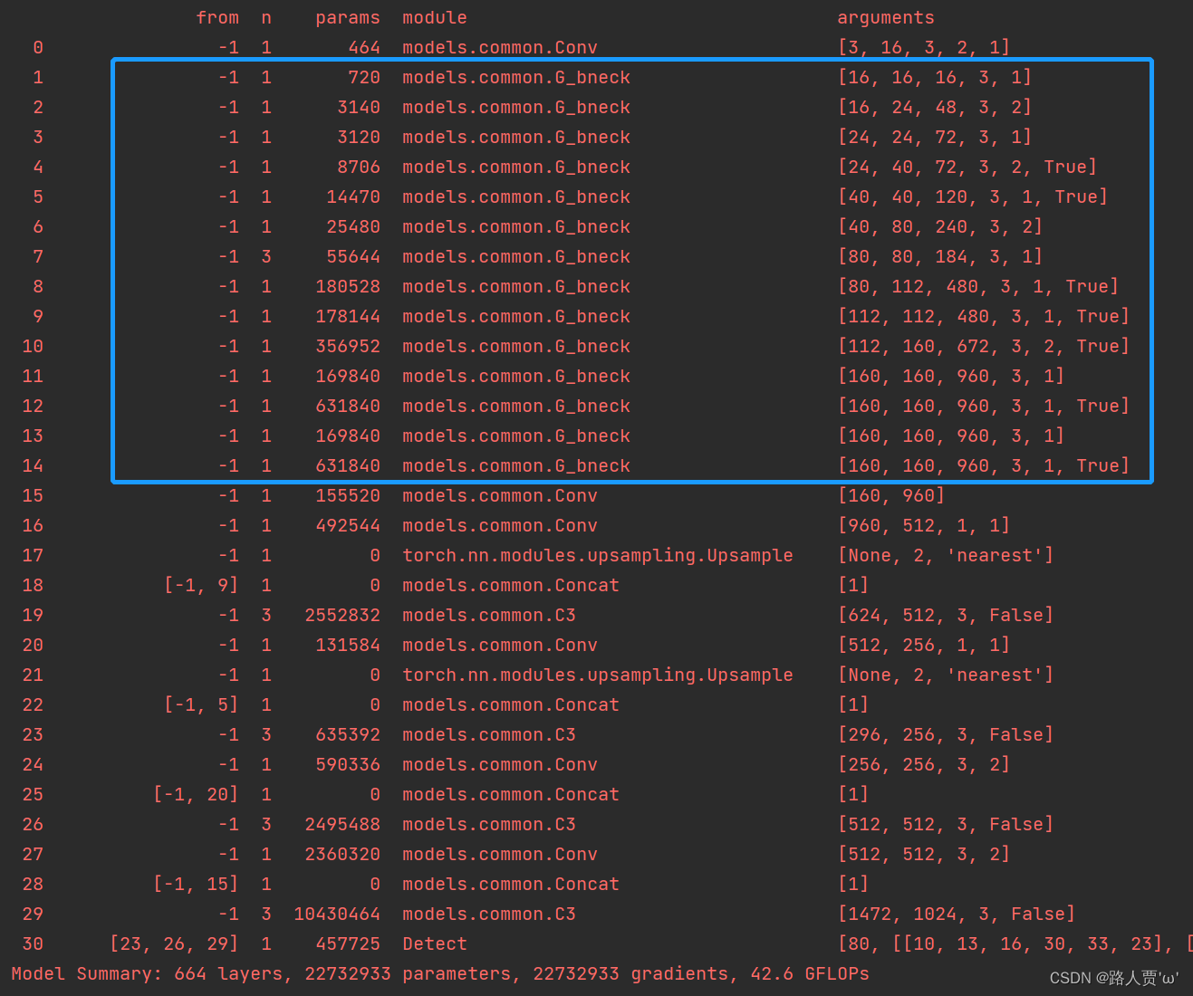
然后运行yolo.py
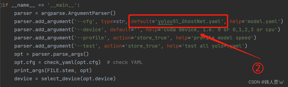
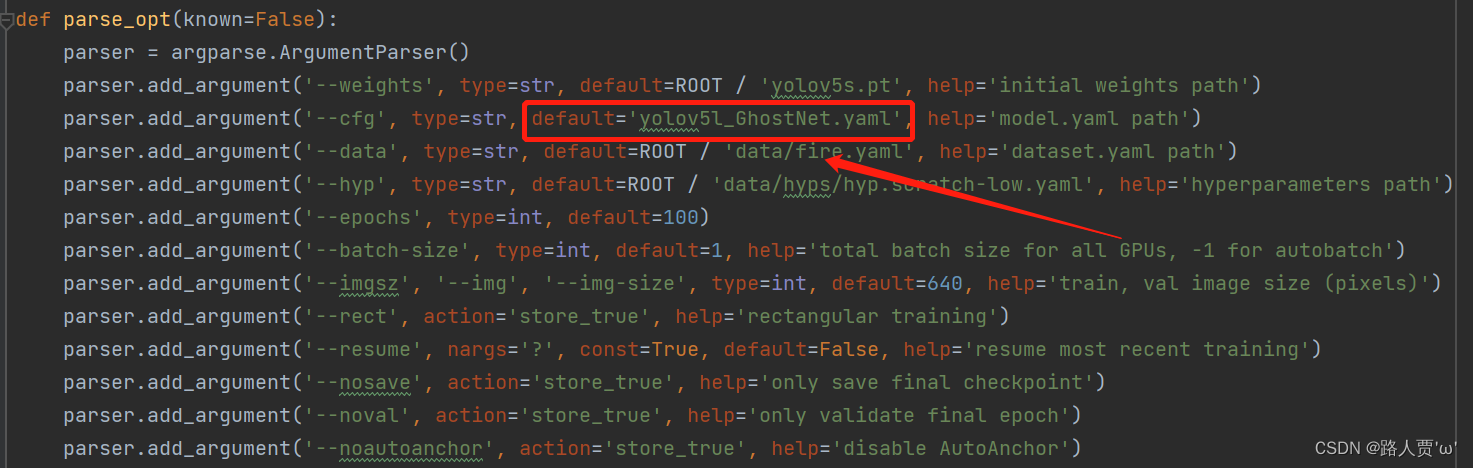
这样就成功啦~ 第⑤步:修改train.py中 ‘–cfg’默认参数我们先找到 train.py 文件的parse_opt函数,然后将第二行**‘–cfg’的 default改为’yolo5l_GhostNet.yaml’**,然后就可以开始训练啦~
MobileViTv1详细解读 MobileViTv1结构详解 一、MobileViT v1介绍
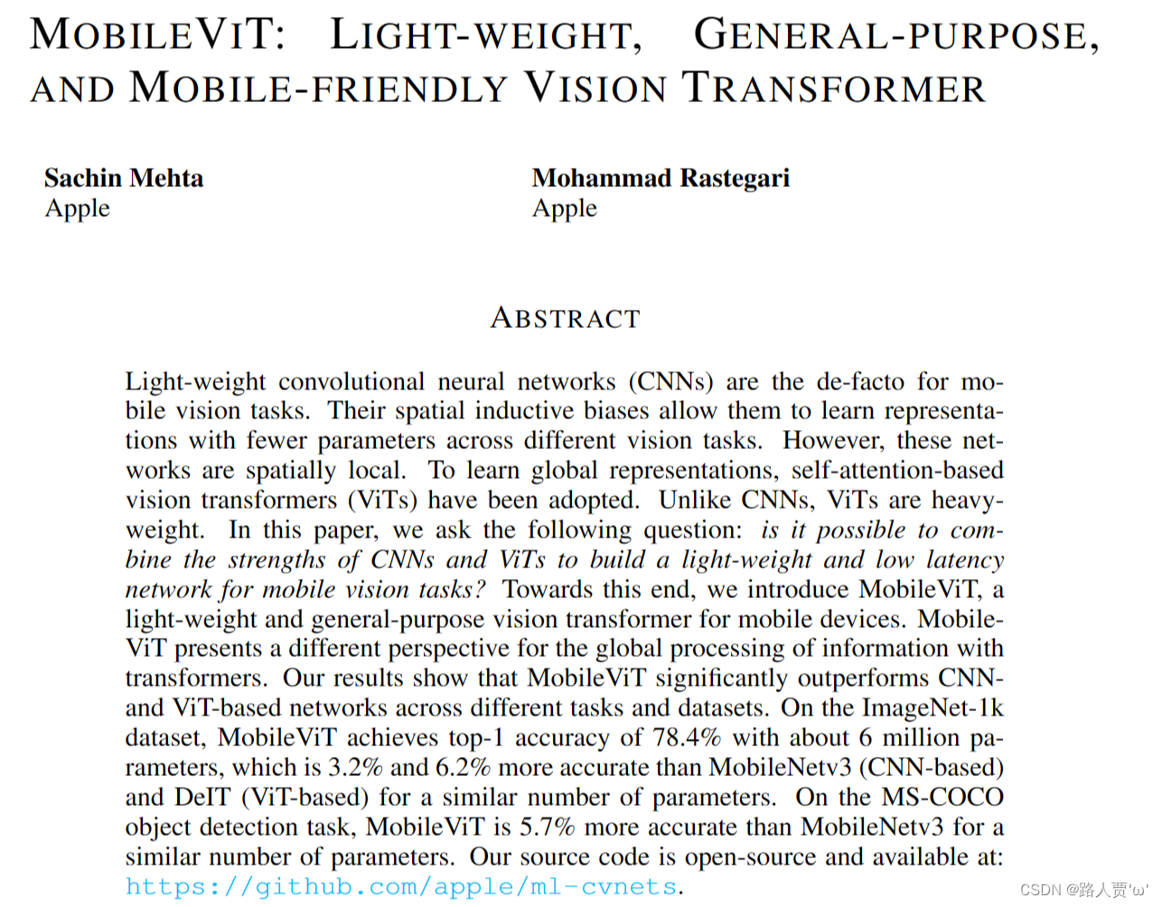
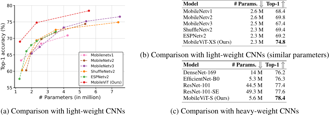
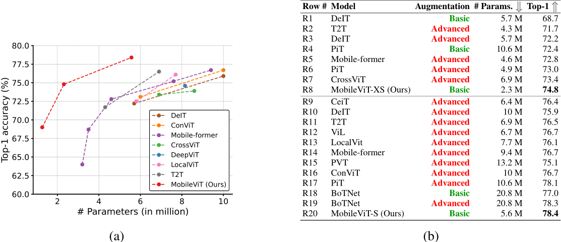
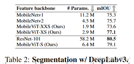
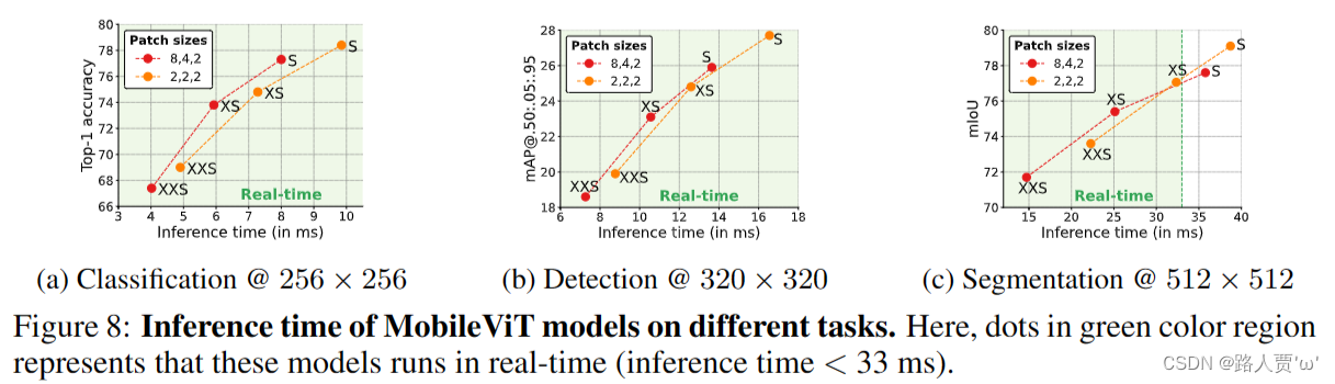
MobileViT网络是由苹果公司提出了一种轻量级的、通用的移动设备 vision transformer,将CNN和ViT的优势相结合,提高了在移动视觉任务中的性能。 以往的研究主要集中在轻量级卷积神经网络和自注意力ViTs,其中CNN具有局部感知性,参数较少,ViTs具有全局感知性,但参数较多。然而,这些方法在移动视觉任务中存在一些问题,如性能不够理想、延迟较高等。 本篇论文提出了MobileViT的研究方法,将transformers作为卷积的方式进行全局信息处理,实现了轻量级和低延迟的移动视觉任务网络。 研究结果表明,MobileViT在不同任务和数据集上明显优于基于CNN和ViT的网络。在ImageNet-1k数据集上取得了最佳结果。 1.2 网络结构
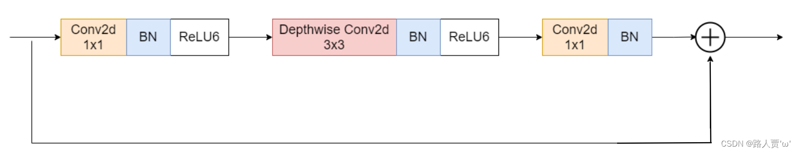
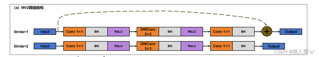
上面那个图展示就是标准视觉ViT模型,下面就是今天要介绍的MobileViT的网络结构。 主要由MV2和MobileViTblock两个模块组成,下面我们来介绍下这两个模块: (1)MV2MV2就是MobileNet v2(直通车:【轻量化网络系列(2)】MobileNetV2论文超详细解读(翻译 +学习笔记+代码实现))里面Inverted Residual Block,即下面的图所示的结构。
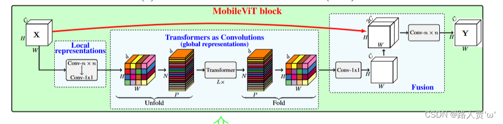
图中MV2是当stride等于1时的MV2结构,上图中标有向下箭头的MV2结构代表stride等于2的情况,即需要进行下采样。 (2)MobileViTblock
首先将特征图通过一个卷积层,卷积核大小为n×n,然后再通过一个卷积核大小为1×1的卷积层进行通道调整。 接着依次通过Unfold、Transformer、Fold结构进行全局特征建模,然后再通过一个卷积核大小为1×1的卷积层将通道调整为原始大小。 接着通过shortcut捷径分支与原始输入特征图按通道concat拼接。 最后再通过一个卷积核大小为n×n的卷积层进行特征融合得到最终的输出。 1.3 实验 (1)和CNN对比
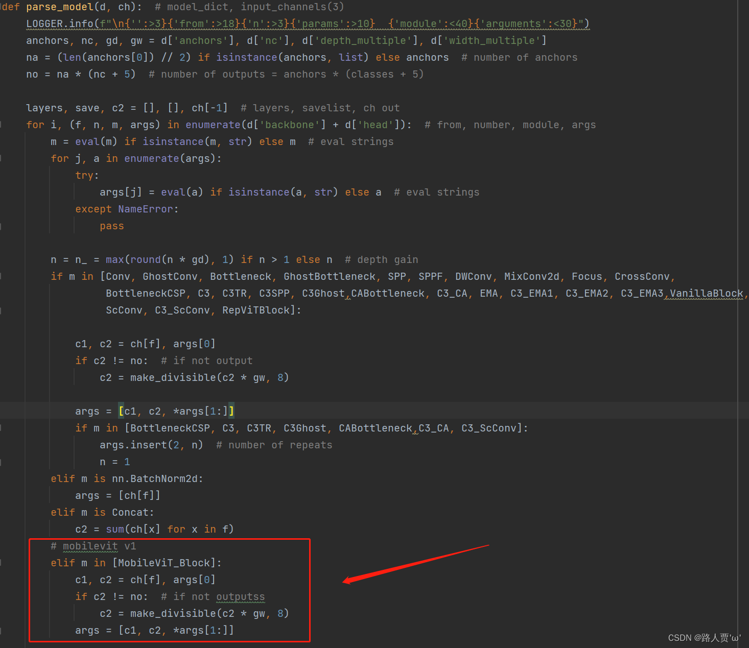
将以下代码复制粘贴到common.py文件的末尾 from einops import rearrange import torch import torch.nn as nn # Transformer Attention模块定义 class TAttention(nn.Module): def __init__(self, dim, heads=8, dim_head=64, dropout=0.): super().__init__() inner_dim = dim_head * heads project_out = not (heads == 1 and dim_head == dim) self.heads = heads self.scale = dim_head ** -0.5 self.attend = nn.Softmax(dim=-1) self.to_qkv = nn.Linear(dim, inner_dim * 3, bias=False) self.to_out = nn.Sequential( nn.Linear(inner_dim, dim), nn.Dropout(dropout) ) if project_out else nn.Identity() def forward(self, x): qkv = self.to_qkv(x).chunk(3, dim=-1) q, k, v = map(lambda t: rearrange(t, 'b p n (h d) -> b p h n d', h=self.heads), qkv) dots = torch.matmul(q, k.transpose(-1, -2)) * self.scale attn = self.attend(dots) out = torch.matmul(attn, v) out = rearrange(out, 'b p h n d -> b p n (h d)') return self.to_out(out) # MobileViT模块定义 class MoblieTrans(nn.Module): def __init__(self, dim, depth, heads, dim_head, mlp_dim, dropout=0.): super().__init__() self.layers = nn.ModuleList([]) for _ in range(depth): self.layers.append(nn.ModuleList([ PreNorm(dim, TAttention(dim, heads, dim_head, dropout)), PreNorm(dim, FeedForward(dim, mlp_dim, dropout)) ])) def forward(self, x): for attn, ff in self.layers: x = attn(x) + x x = ff(x) + x return x # MobileViT Block定义 class MV2B(nn.Module): def __init__(self, ch_in, ch_out, stride=1, expansion=4): super().__init__() self.stride = stride assert stride in [1, 2] hidden_dim = int(ch_in * expansion) self.use_res_connect = self.stride == 1 and ch_in == ch_out if expansion == 1: self.conv = nn.Sequential( nn.Conv2d(hidden_dim, hidden_dim, 3, stride, 1, groups=hidden_dim, bias=False), nn.BatchNorm2d(hidden_dim), nn.SiLU(), nn.Conv2d(hidden_dim, ch_out, 1, 1, 0, bias=False), nn.BatchNorm2d(ch_out), ) else: self.conv = nn.Sequential( nn.Conv2d(ch_in, hidden_dim, 1, 1, 0, bias=False), nn.BatchNorm2d(hidden_dim), nn.SiLU(), nn.Conv2d(hidden_dim, hidden_dim, 3, stride, 1, groups=hidden_dim, bias=False), nn.BatchNorm2d(hidden_dim), nn.SiLU(), nn.Conv2d(hidden_dim, ch_out, 1, 1, 0, bias=False), nn.BatchNorm2d(ch_out), ) def forward(self, x): if self.use_res_connect: return x + self.conv(x) else: return self.conv(x) # MobileViT Block定义 class MobileViT_Block(nn.Module): def __init__(self, ch_in, dim=64, depth=2, kernel_size=3, patch_size=(2, 2), mlp_dim=int(64 * 2), dropout=0.): super().__init__() self.ph, self.pw = patch_size self.conv1 = conv_nxn_bn(ch_in, ch_in, kernel_size) self.conv2 = conv_1x1_bn(ch_in, dim) self.transformer = MoblieTrans(dim, depth, 4, 8, mlp_dim, dropout) self.conv3 = conv_1x1_bn(dim, ch_in) self.conv4 = conv_nxn_bn(2 * ch_in, ch_in, kernel_size) def forward(self, x): y = x.clone() # Local representations x = self.conv1(x) x = self.conv2(x) # Global representations _, _, h, w = x.shape x = rearrange(x, 'b d (h ph) (w pw) -> b (ph pw) (h w) d', ph=self.ph, pw=self.pw) x = self.transformer(x) x = rearrange(x, 'b (ph pw) (h w) d -> b d (h ph) (w pw)', h=h // self.ph, w=w // self.pw, ph=self.ph, pw=self.pw) x = self.conv3(x) x = torch.cat((x, y), 1) x = self.conv4(x) return x # 1x1卷积层+BatchNorm+SiLU激活函数 def conv_1x1_bn(ch_in, ch_out): return nn.Sequential( nn.Conv2d(ch_in, ch_out, 1, 1, 0, bias=False), nn.BatchNorm2d(ch_out), nn.SiLU() ) # nxn卷积层+BatchNorm+SiLU激活函数 def conv_nxn_bn(ch_in, ch_out, kernal_size=3, stride=1): return nn.Sequential( nn.Conv2d(ch_in, ch_out, kernal_size, stride, 1, bias=False), nn.BatchNorm2d(ch_out), nn.SiLU() ) # LayerNormalization + Function模块 class PreNorm(nn.Module): def __init__(self, dim, fn): super().__init__() self.norm = nn.LayerNorm(dim) self.fn = fn def forward(self, x, **kwargs): return self.fn(self.norm(x), **kwargs) # Feed Forward模块 class FeedForward(nn.Module): def __init__(self, dim, hidden_dim, dropout=0.): super().__init__() self.net = nn.Sequential( nn.Linear(dim, hidden_dim), nn.SiLU(), nn.Dropout(dropout), nn.Linear(hidden_dim, dim), nn.Dropout(dropout) ) def forward(self, x): return self.net(x) 第②步:修改yolo.py文件再来修改yolo.py,在parse_model函数中找到 elif m is Concat: 语句,在其后面加上下面代码: # mobilevit v1 elif m in [MobileViT_Block]: c1, c2 = ch[f], args[0] if c2 != no: # if not outputss c2 = make_divisible(c2 * gw, 8) args = [c1, c2, *args[1:]]如下图所示:
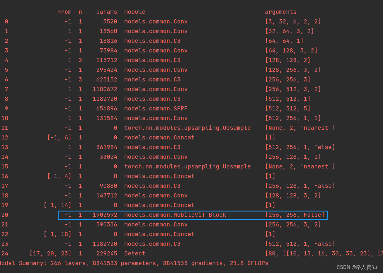
yaml文件配置完整代码如下: # YOLOv5 🚀 by Ultralytics, GPL-3.0 license # Parameters nc: 80 # number of classes depth_multiple: 0.33 # model depth multiple width_multiple: 0.50 # layer channel multiple anchors: - [10,13, 16,30, 33,23] # P3/8 - [30,61, 62,45, 59,119] # P4/16 - [116,90, 156,198, 373,326] # P5/32 # YOLOv5 v6.0 backbone backbone: # [from, number, module, args] [[-1, 1, Conv, [64, 6, 2, 2]], # 0-P1/2 [-1, 1, Conv, [128, 3, 2]], # 1-P2/4 [-1, 3, C3, [128]], [-1, 1, Conv, [256, 3, 2]], # 3-P3/8 [-1, 6, C3, [256]], [-1, 1, Conv, [512, 3, 2]], # 5-P4/16 [-1, 9, C3, [512]], [-1, 1, Conv, [1024, 3, 2]], # 7-P5/32 [-1, 3, C3, [1024]], [-1, 1, SPPF, [1024, 5]], # 9 ] # YOLOv5 v6.0 head head: [[-1, 1, Conv, [512, 1, 1]], [-1, 1, nn.Upsample, [None, 2, 'nearest']], [[-1, 6], 1, Concat, [1]], # cat backbone P4 [-1, 3, C3, [512, False]], # 13 [-1, 1, Conv, [256, 1, 1]], [-1, 1, nn.Upsample, [None, 2, 'nearest']], [[-1, 4], 1, Concat, [1]], # cat backbone P3 [-1, 3, C3, [256, False]], # 17 (P3/8-small) [-1, 1, Conv, [256, 3, 2]], [[-1, 14], 1, Concat, [1]], # cat head P4 [-1, 3, MobileViT_Block, [512, False]], # 20 (P4/16-medium) [-1, 1, Conv, [512, 3, 2]], [[-1, 10], 1, Concat, [1]], # cat head P5 [-1, 3, C3, [1024, False]], # 23 (P5/32-large) [[17, 20, 23], 1, Detect, [nc, anchors]], # Detect(P3, P4, P5) ] 第④步 验证是否加入成功运行yolo.py
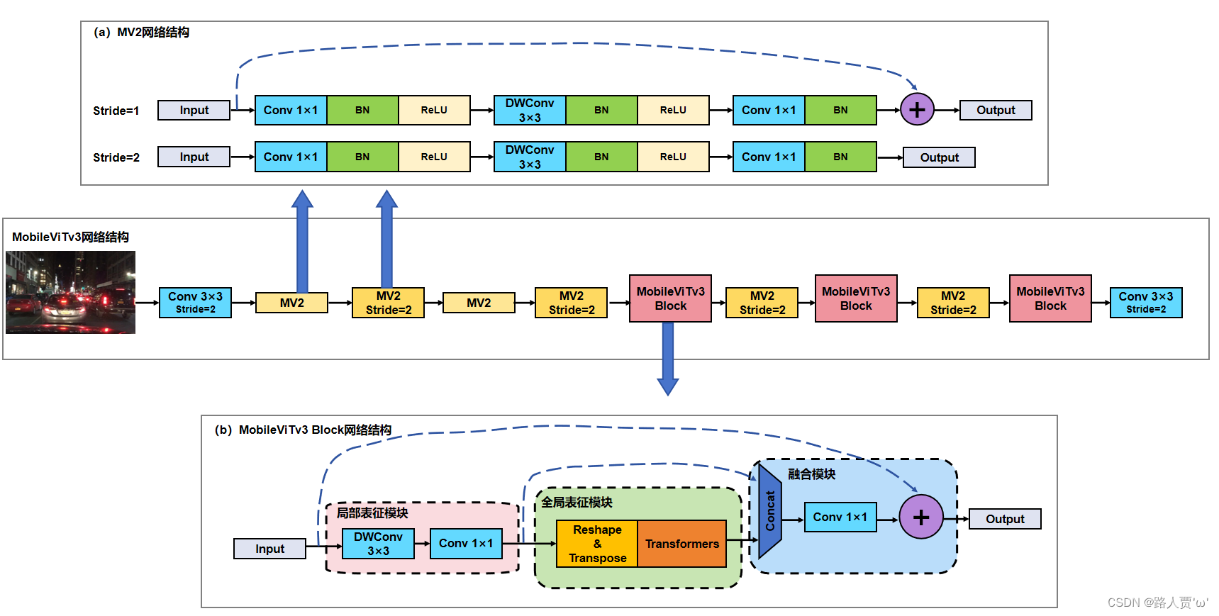
论文解析 一、MobileViT v3介绍 在之前的研究中,**CNN模型足够轻量化但是精准度有待提高**,**ViT模型具有较好的识别能力但是模型参数量大,计算复杂**,都不能满足移动端实时高效检测的需求。 **MobileViT**模型是2021年苹果公司提出的基于轻量化的ViT模型,该模型**既具备ViT模型准确检测的优越性能**,**也具备CNN模型的轻量化优点**,能极大程度上减少模型参数,对移动端友好,具备部署于移动设备的可能性。MobileViT v****3是该公司2022年9月推出的第3个版本,该模型相较于初始版本有以下四个改进: 首先,将3×3卷积层替换为1×1卷积层;第二,将局部表示块和全局表示块的特征融合在一起;第三,在生成MobileViT Block输出之前,在融合块中添加输入特征作为最后一步;最后,在局部表示块中,将普通的3×3卷积层替换为深度3×3卷积层。MobileViTv3网络结构图如下所示:
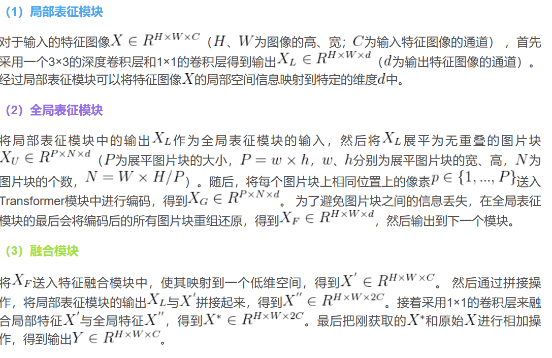
模型预测处理过程如下: (1)将输入图像连接3×3标准卷积并做2倍下采样;之后通过5个MV2模块(如图(a)所示),其中步长为1的MV2模块进行特征提取,步长为2的MV2模块做2倍下采样; (2)将得到的特征图间隔传入MobileViTV3 Block(如图(b)所示)和步长为2的MV2模块; (3)接着使用3×3标准卷积进行通道压缩; (4)最后进行全局平均池化来获取预测结果 。 MobileViT v3 Block模块是MobileViT v3核心部分,由局部表征模块、全局表征模块、融合模块三部分组成,具体介绍如下:
首先,定义卷积层。 分为1×1卷积层和n×n(n=3)卷积层 def conv_1x1_bn(inp, oup): return nn.Sequential( nn.Conv2d(inp, oup, 1, 1, 0, bias=False), nn.BatchNorm2d(oup), nn.SiLU() ) def conv_nxn_bn(inp, oup, kernal_size=3, stride=1): return nn.Sequential( nn.Conv2d(inp, oup, kernal_size, stride, 1, bias=False), nn.BatchNorm2d(oup), nn.SiLU() )接着,构造ViT模块。 Transformer Encoder模块中编码 class PreNorm(nn.Module): def __init__(self, dim, fn): super().__init__() self.norm = nn.LayerNorm(dim) self.fn = fn # mg def forward(self, x, **kwargs): return self.fn(self.norm(x), **kwargs) class Attention(nn.Module): def __init__(self, dim, heads=8, dim_head=64, dropout=0.): super().__init__() inner_dim = dim_head * heads project_out = not (heads == 1 and dim_head == dim) self.heads = heads self.scale = dim_head ** -0.5 self.attend = nn.Softmax(dim = -1) self.to_qkv = nn.Linear(dim, inner_dim * 3, bias = False) self.to_out = nn.Sequential( nn.Linear(inner_dim, dim), nn.Dropout(dropout)# mg ) if project_out else nn.Identity() def forward(self, x): qkv = self.to_qkv(x).chunk(3, dim=-1) q, k, v = map(lambda t: rearrange(t, 'b p n (h d) -> b p h n d', h = self.heads), qkv) dots = torch.matmul(q, k.transpose(-1, -2)) * self.scale attn = self.attend(dots) out = torch.matmul(attn, v) out = rearrange(out, 'b p h n d -> b p n (h d)') return self.to_out(out) class FeedForward(nn.Module): def __init__(self, dim, hidden_dim, dropout=0.): super().__init__() self.net = nn.Sequential( nn.Linear(dim, hidden_dim), nn.SiLU(), nn.Dropout(dropout), nn.Linear(hidden_dim, dim), nn.Dropout(dropout) ) def forward(self, x): return self.net(x) class MBTransformer(nn.Module): def __init__(self, dim, depth, heads, dim_head, mlp_dim, dropout=0.): super().__init__() self.layers = nn.ModuleList([]) for _ in range(depth): self.layers.append(nn.ModuleList([ PreNorm(dim, Attention(dim, heads, dim_head, dropout)), PreNorm(dim, FeedForward(dim, mlp_dim, dropout)) ])) def forward(self, x): for attn, ff in self.layers: x = attn(x) + x x = ff(x) + x return x然后,MV2模块。
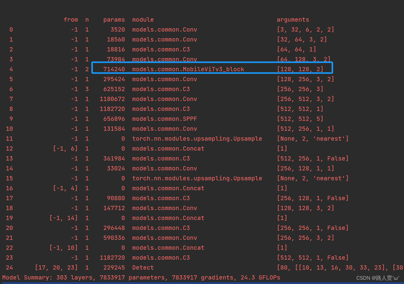
分为stride=1和stride=2两种。 class MV2Block(nn.Module): def __init__(self, inp, oup, stride=1, expansion=4): super().__init__() self.stride = stride assert stride in [1, 2] hidden_dim = int(inp * expansion) self.use_res_connect = self.stride == 1 and inp == oup if expansion == 1: self.conv = nn.Sequential( # dw nn.Conv2d(hidden_dim, hidden_dim, 3, stride, 1, groups=hidden_dim, bias=False), nn.BatchNorm2d(hidden_dim), nn.SiLU(), # pw-linear nn.Conv2d(hidden_dim, oup, 1, 1, 0, bias=False), nn.BatchNorm2d(oup), ) else: self.conv = nn.Sequential( # pw nn.Conv2d(inp, hidden_dim, 1, 1, 0, bias=False), nn.BatchNorm2d(hidden_dim), nn.SiLU(), # dw nn.Conv2d(hidden_dim, hidden_dim, 3, stride, 1, groups=hidden_dim, bias=False), nn.BatchNorm2d(hidden_dim), nn.SiLU(), # pw-linear nn.Conv2d(hidden_dim, oup, 1, 1, 0, bias=False), nn.BatchNorm2d(oup), ) def forward(self, x): if self.use_res_connect: return x + self.conv(x) else: return self.conv(x)最后,核心模块 MobileViTv3_block。 介绍部分看上面就行~ class MobileViTv3_block(nn.Module): def __init__(self, channel, dim, depth=2, kernel_size=3, patch_size=(2, 2), mlp_dim=int(64*2), dropout=0.): super().__init__() self.ph, self.pw = patch_size self.mv01 = MV2Block(channel, channel) self.conv1 = conv_nxn_bn(channel, channel, kernel_size) self.conv3 = conv_1x1_bn(dim, channel) self.conv2 = conv_1x1_bn(channel, dim) self.transformer = MBTransformer(dim, depth, 4, 8, mlp_dim, dropout) self.conv4 = conv_nxn_bn(2 * channel, channel, kernel_size) def forward(self, x): y = x.clone() x = self.conv1(x) x = self.conv2(x) z = x.clone() _, _, h, w = x.shape x = rearrange(x, 'b d (h ph) (w pw) -> b (ph pw) (h w) d', ph=self.ph, pw=self.pw) x = self.transformer(x) x = rearrange(x, 'b (ph pw) (h w) d -> b d (h ph) (w pw)', h=h//self.ph, w=w//self.pw, ph=self.ph, pw=self.pw) x = self.conv3(x) x = torch.cat((x, z), 1) x = self.conv4(x) x = x + y x = self.mv01(x) return x以下是完整代码: 将以下代码复制粘贴到common.py文件的末尾 from einops import rearrange def conv_1x1_bn(inp, oup): return nn.Sequential( nn.Conv2d(inp, oup, 1, 1, 0, bias=False), nn.BatchNorm2d(oup), nn.SiLU() ) def conv_nxn_bn(inp, oup, kernal_size=3, stride=1): return nn.Sequential( nn.Conv2d(inp, oup, kernal_size, stride, 1, bias=False), nn.BatchNorm2d(oup), nn.SiLU() ) class PreNorm(nn.Module): def __init__(self, dim, fn): super().__init__() self.norm = nn.LayerNorm(dim) self.fn = fn # mg def forward(self, x, **kwargs): return self.fn(self.norm(x), **kwargs) class Attention(nn.Module): def __init__(self, dim, heads=8, dim_head=64, dropout=0.): super().__init__() inner_dim = dim_head * heads project_out = not (heads == 1 and dim_head == dim) self.heads = heads self.scale = dim_head ** -0.5 self.attend = nn.Softmax(dim = -1) self.to_qkv = nn.Linear(dim, inner_dim * 3, bias = False) self.to_out = nn.Sequential( nn.Linear(inner_dim, dim), nn.Dropout(dropout)# mg ) if project_out else nn.Identity() def forward(self, x): qkv = self.to_qkv(x).chunk(3, dim=-1) q, k, v = map(lambda t: rearrange(t, 'b p n (h d) -> b p h n d', h = self.heads), qkv) dots = torch.matmul(q, k.transpose(-1, -2)) * self.scale attn = self.attend(dots) out = torch.matmul(attn, v) out = rearrange(out, 'b p h n d -> b p n (h d)') return self.to_out(out) class FeedForward(nn.Module): def __init__(self, dim, hidden_dim, dropout=0.): super().__init__() self.net = nn.Sequential( nn.Linear(dim, hidden_dim), nn.SiLU(), nn.Dropout(dropout), nn.Linear(hidden_dim, dim), nn.Dropout(dropout) ) def forward(self, x): return self.net(x) class MBTransformer(nn.Module): def __init__(self, dim, depth, heads, dim_head, mlp_dim, dropout=0.): super().__init__() self.layers = nn.ModuleList([]) for _ in range(depth): self.layers.append(nn.ModuleList([ PreNorm(dim, Attention(dim, heads, dim_head, dropout)), PreNorm(dim, FeedForward(dim, mlp_dim, dropout)) ])) def forward(self, x): for attn, ff in self.layers: x = attn(x) + x x = ff(x) + x return x class MV2Block(nn.Module): def __init__(self, inp, oup, stride=1, expansion=4): super().__init__() self.stride = stride assert stride in [1, 2] hidden_dim = int(inp * expansion) self.use_res_connect = self.stride == 1 and inp == oup if expansion == 1: self.conv = nn.Sequential( # dw nn.Conv2d(hidden_dim, hidden_dim, 3, stride, 1, groups=hidden_dim, bias=False), nn.BatchNorm2d(hidden_dim), nn.SiLU(), # pw-linear nn.Conv2d(hidden_dim, oup, 1, 1, 0, bias=False), nn.BatchNorm2d(oup), ) else: self.conv = nn.Sequential( # pw nn.Conv2d(inp, hidden_dim, 1, 1, 0, bias=False), nn.BatchNorm2d(hidden_dim), nn.SiLU(), # dw nn.Conv2d(hidden_dim, hidden_dim, 3, stride, 1, groups=hidden_dim, bias=False), nn.BatchNorm2d(hidden_dim), nn.SiLU(), # pw-linear nn.Conv2d(hidden_dim, oup, 1, 1, 0, bias=False), nn.BatchNorm2d(oup), ) def forward(self, x): if self.use_res_connect: return x + self.conv(x) else: return self.conv(x) class MobileViTv3_block(nn.Module): def __init__(self, channel, dim, depth=2, kernel_size=3, patch_size=(2, 2), mlp_dim=int(64*2), dropout=0.): super().__init__() self.ph, self.pw = patch_size self.mv01 = MV2Block(channel, channel) self.conv1 = conv_nxn_bn(channel, channel, kernel_size) self.conv3 = conv_1x1_bn(dim, channel) self.conv2 = conv_1x1_bn(channel, dim) self.transformer = MBTransformer(dim, depth, 4, 8, mlp_dim, dropout) self.conv4 = conv_nxn_bn(2 * channel, channel, kernel_size) def forward(self, x): y = x.clone() x = self.conv1(x) x = self.conv2(x) z = x.clone() _, _, h, w = x.shape x = rearrange(x, 'b d (h ph) (w pw) -> b (ph pw) (h w) d', ph=self.ph, pw=self.pw) x = self.transformer(x) x = rearrange(x, 'b (ph pw) (h w) d -> b d (h ph) (w pw)', h=h//self.ph, w=w//self.pw, ph=self.ph, pw=self.pw) x = self.conv3(x) x = torch.cat((x, z), 1) x = self.conv4(x) x = x + y x = self.mv01(x) return x 第②步:修改yolo.py文件再来修改yolo.py,在parse_model函数中找到 elif m is Concat: 语句,在其后面加上下面代码: elif m in [MobileViTv3_block]: c1, c2 = ch[f], args[0] if c2 != no: c2 = make_divisible(c2 * gw, 8) args = [c1, c2] if m in [MobileViTv3_block]: args.insert(2, n) n = 1 第③步:创建自定义的yaml文件yaml文件配置完整代码如下: # YOLOv5 🚀 by Ultralytics, GPL-3.0 license # Parameters nc: 80 # number of classes depth_multiple: 0.33 # model depth multiple width_multiple: 0.50 # layer channel iscyy multiple anchors: - [10,13, 16,30, 33,23] # P3/8 - [30,61, 62,45, 59,119] # P4/16 - [116,90, 156,198, 373,326] # P5/32 # YOLOv5 v6.0 backbone backbone: # [from, number, module, args] [[-1, 1, Conv, [64, 6, 2, 2]], # 0-P1/2 [-1, 1, Conv, [128, 3, 2]], # 1-P2/4 [-1, 3, C3, [128]], [-1, 1, Conv, [256, 3, 2]], # 3-P3/8 [-1, 6, MobileViTv3_block, [256]], [-1, 1, Conv, [512, 3, 2]], # 5-P4/16 [-1, 9, C3, [512]], [-1, 1, Conv, [1024, 3, 2]], # 7-P5/32 [-1, 3, C3, [1024]], [-1, 1, SPPF, [1024, 5]], # 9 ] # YOLOv5 v6.0 head head: [[-1, 1, Conv, [512, 1, 1]], [-1, 1, nn.Upsample, [None, 2, 'nearest']], [[-1, 6], 1, Concat, [1]], # cat backbone P4 [-1, 3, C3, [512, False]], # 13 [-1, 1, Conv, [256, 1, 1]], [-1, 1, nn.Upsample, [None, 2, 'nearest']], [[-1, 4], 1, Concat, [1]], # cat backbone P3 [-1, 3, C3, [256, False]], # 17 (P3/8-small) [-1, 1, Conv, [256, 3, 2]], [[-1, 14], 1, Concat, [1]], # cat head P4 [-1, 3, C3, [512, False]], # 20 (P4/16-medium) [-1, 1, Conv, [512, 3, 2]], [[-1, 10], 1, Concat, [1]], # cat head P5 [-1, 3, C3, [1024, False]], # 23 (P5/32-large) [[17, 20, 23], 1, Detect, [nc, anchors]], # Detect(P3, P4, P5) ] 第④步 验证是否加入成功运行yolo.py
详细解读
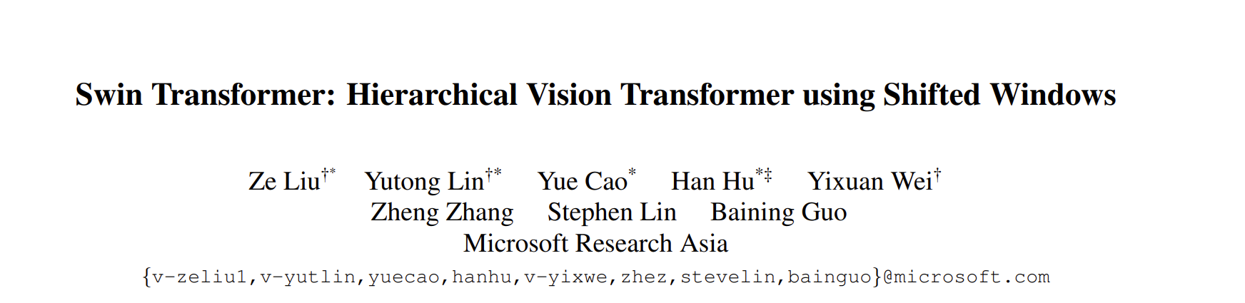
论文地址:https://arxiv.org/pdf/2103.14030.pdf 代码地址:https://github.com/microsoft/Swin-Transformer 本文介绍了一种新的视觉Transformer,称为Swin Transformer,它可以作为计算机视觉通用的骨干网络。从语言到视觉的转换中,适应Transformer所面临的挑战源于两个领域之间的差异,如视觉实体尺度的巨大变化和图像中像素的高分辨率与文本中单词的差异。为了解决这些差异,我们提出了一种分层Transformer,其表示是通过Shifted窗口计算的。Shifted窗口方案通过将自注意计算限制在非重叠的本地窗口内,同时允许跨窗口连接,从而提高了效率。这种分层架构具有在不同尺度下进行建模的灵活性,并且与图像大小的计算复杂度呈线性关系。这些特性使Swin Transformer与广泛的视觉任务兼容,包括图像分类(在ImageNet-1K上的87.3的top-1准确率)和密集预测任务,如物体检测(在COCO测试中的58.7 box AP和51.1 mask AP)和语义分割(在ADE20K val上的53.5 mIoU)。它的性能在COCO上比先前的最先进水平提高了2.7个box AP和2.6个mask AP,在ADE20K上提高了3.2个mIoU,展示了基于Transformer的模型作为视觉骨干的潜力。分层设计和Shifted窗口方法对于所有MLP架构也证明是有益的。 Swin Transformer 对比 Vision TransformerSwin Transformer和Vision Transformer都是基于Transformer模型的变种,但它们在具体实现和应用上还是有些区别的。 输入结构不同 Vision Transformer将输入的图像分成若干个小块,并将每个块看作一个序列,然后通过Transformer编码器对这些序列进行处理。而Swin Transformer则是将整张图像看作一个序列,通过新型的局部注意力机制进行处理。注意力机制不同 在Vision Transformer中,自注意力机制被应用于处理输入序列。在这种机制下,每个位置都会与序列中的其他位置进行交互,从而获得全局的上下文信息。而在Swin Transformer中,引入了局部注意力机制,它只关注相邻的一部分位置,从而大幅减少了计算复杂度。计算复杂度不同 Swin Transformer通过局部注意力机制和跨阶段连接(Cross-Stage Connection)等技术,使得在处理大型图像时,计算复杂度明显优于Vision Transformer。同时,在参数数量相同时,Swin Transformer的表现也更优秀。
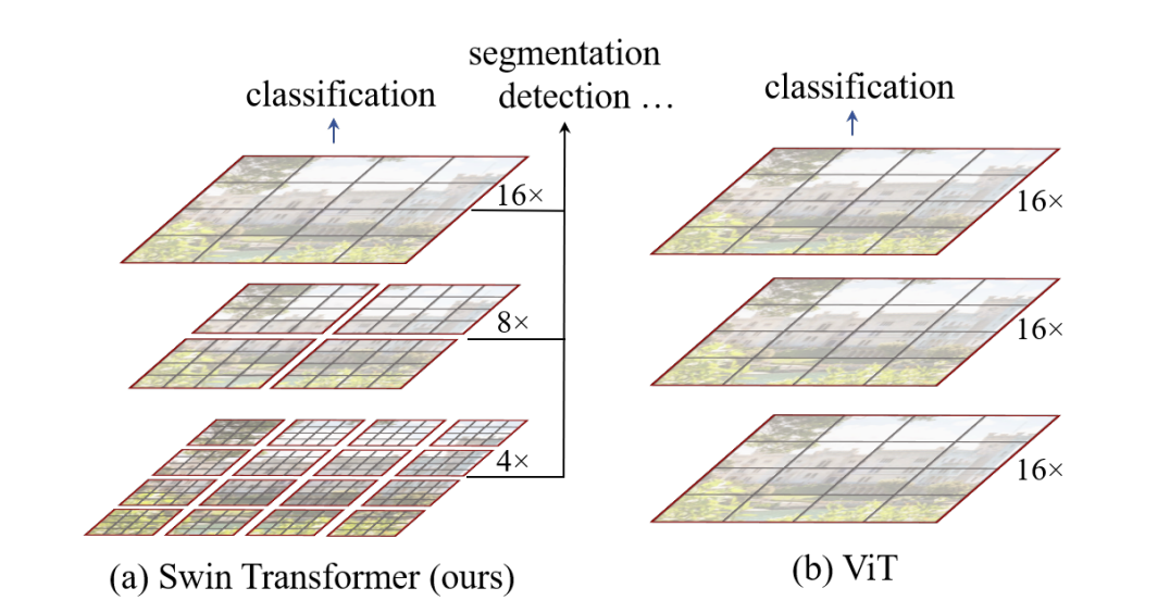
(a)提出的Swin Transformer通过在深层中合并图像块(灰色表示)来构建分层特征映射,并且由于仅在每个局部窗口内计算自注意力(红色表示),因此具有与输入图像大小线性的计算复杂度。因此,它可以作为图像分类和密集识别任务的通用骨干。(b)相比之下,以往的Vision Transformer生成单个低分辨率的特征映射,并且由于在全局计算自注意力(红色表示),因此其计算复杂度与输入图像大小呈二次关系。 Swin Transformer 结构
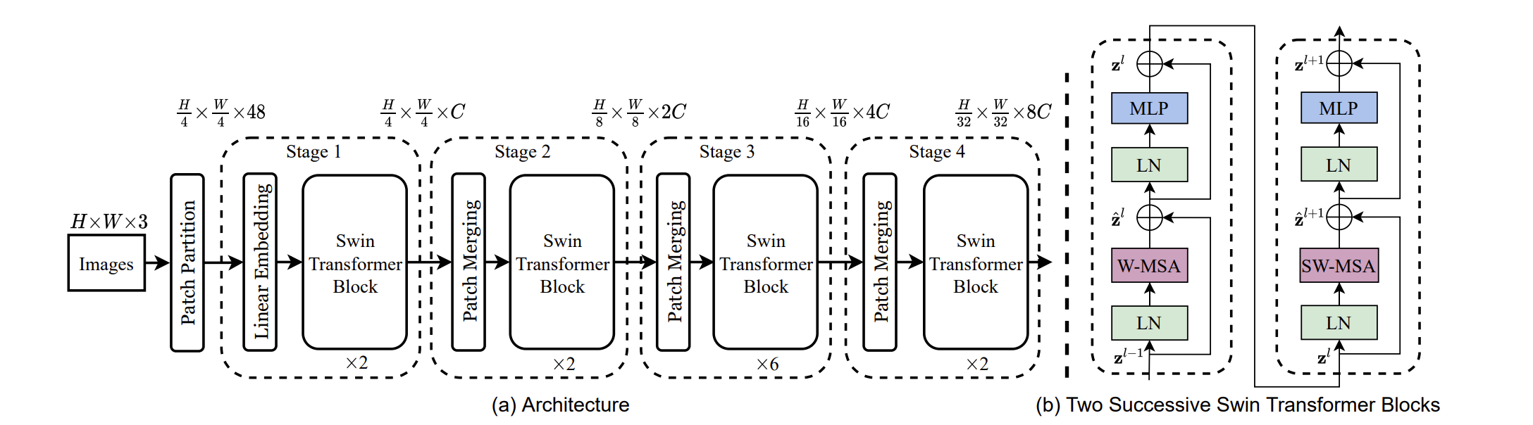
(a) Swin Transformer(Swin-T)的架构; (b) 两个连续的Swin Transformer块。W-MSA和SW-MSA是带有常规和位移窗口配置的多头自注意力模块。 不同尺寸的 Swin Transformer 结构参数对比
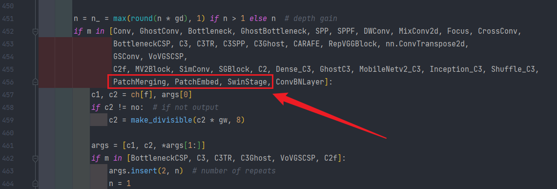
详细的架构规格说明 在 YOLO 项目中添加 SwinTransformer 主干的方式 第一步在 common.py 中添加如下的代码: def drop_path_f(x, drop_prob: float = 0., training: bool = False): """ Drop paths (Stochastic Depth) per sample (when applied in main path of residual blocks). Args: x (Tensor): 输入张量。 drop_prob (float): 丢弃的概率,范围为0到1。 training (bool): 模型是否处于训练模式。 Returns: Tensor: 经过Drop Path操作后的张量。 """ if drop_prob == 0. or not training: # 如果丢弃概率为0或模型不处于训练模式,则直接返回输入张量 return x keep_prob = 1 - drop_prob # 计算保留的概率 shape = (x.shape[0],) + (1,) * (x.ndim - 1) # 确保适用于不同维度的张量,而不仅仅是2D卷积网络 random_tensor = keep_prob + torch.rand(shape, dtype=x.dtype, device=x.device) random_tensor.floor_() # 将随机张量二值化,以确定要保留的路径 output = x.div(keep_prob) * random_tensor return output class DropPath(nn.Module): """ 在应用于残差块的主路径中每个样本的Drop Path(随机深度). """ def __init__(self, drop_prob=None): """ 初始化DropPath模块。 Args: drop_prob (float): 丢弃的概率,范围为0到1。 """ super(DropPath, self).__init__() self.drop_prob = drop_prob def forward(self, x): """ 在输入张量的主路径中应用Drop Path操作。 Args: x (Tensor): 输入张量。 Returns: Tensor: 经过Drop Path操作后的张量。 """ return drop_path_f(x, self.drop_prob, self.training) class Mlp(nn.Module): """ MLP as used in Vision Transformer, MLP-Mixer and related networks """ def __init__(self, in_features, hidden_features=None, out_features=None, act_layer=nn.GELU, drop=0.): super().__init__() out_features = out_features or in_features hidden_features = hidden_features or in_features # 第一个全连接层,输入特征数为in_features,输出特征数为hidden_features self.fc1 = nn.Linear(in_features, hidden_features) # 激活函数,默认为GELU self.act = act_layer() # 第一个Dropout层,用于防止过拟合 self.drop1 = nn.Dropout(drop) # 第二个全连接层,输入特征数为hidden_features,输出特征数为out_features self.fc2 = nn.Linear(hidden_features, out_features) # 第二个Dropout层,用于防止过拟合 self.drop2 = nn.Dropout(drop) def forward(self, x): # 第一个全连接层的前向传播 x = self.fc1(x) # 应用激活函数 x = self.act(x) # 应用第一个Dropout层 x = self.drop1(x) # 第二个全连接层的前向传播 x = self.fc2(x) # 应用第二个Dropout层 x = self.drop2(x) return x class WindowAttention(nn.Module): r""" 基于窗口的多头自注意力(W-MSA)模块,具有相对位置偏差。 支持位移和非位移窗口。 Args: dim (int): 输入通道的数量。 window_size (tuple[int]): 窗口的高度和宽度。 num_heads (int): 注意力头的数量。 qkv_bias (bool, optional): 如果为True,则向查询、键、值添加可学习的偏置。默认值:True attn_drop (float, optional): 注意力权重的丢弃率。默认值:0.0 proj_drop (float, optional): 输出的丢弃率。默认值:0.0 """ def __init__(self, dim, window_size, num_heads, qkv_bias=True, attn_drop=0., proj_drop=0.): super().__init__() self.dim = dim self.window_size = window_size # [Mh, Mw] self.num_heads = num_heads head_dim = dim // num_heads self.scale = head_dim ** -0.5 # 定义相对位置偏差的参数表 self.relative_position_bias_table = nn.Parameter( torch.zeros((2 * window_size[0] - 1) * (2 * window_size[1] - 1), num_heads)) # [2*Mh-1 * 2*Mw-1, nH] # 为窗口内的每个令牌获取成对的相对位置索引 coords_h = torch.arange(self.window_size[0]) coords_w = torch.arange(self.window_size[1]) coords = torch.stack(torch.meshgrid([coords_h, coords_w], indexing="ij")) # [2, Mh, Mw] coords_flatten = torch.flatten(coords, 1) # [2, Mh*Mw] # [2, Mh*Mw, 1] - [2, 1, Mh*Mw] relative_coords = coords_flatten[:, :, None] - coords_flatten[:, None, :] # [2, Mh*Mw, Mh*Mw] relative_coords = relative_coords.permute(1, 2, 0).contiguous() # [Mh*Mw, Mh*Mw, 2] relative_coords[:, :, 0] += self.window_size[0] - 1 # 从0开始偏移 relative_coords[:, :, 1] += self.window_size[1] - 1 relative_coords[:, :, 0] *= 2 * self.window_size[1] - 1 relative_position_index = relative_coords.sum(-1) # [Mh*Mw, Mh*Mw] self.register_buffer("relative_position_index", relative_position_index) self.qkv = nn.Linear(dim, dim * 3, bias=qkv_bias) self.attn_drop = nn.Dropout(attn_drop) self.proj = nn.Linear(dim, dim) self.proj_drop = nn.Dropout(proj_drop) nn.init.trunc_normal_(self.relative_position_bias_table, std=.02) self.softmax = nn.Softmax(dim=-1) def forward(self, x, mask: Optional[torch.Tensor] = None): """ Args: x: 输入特征,形状为 (num_windows*B, Mh*Mw, C) mask: (0/-inf)形状为 (num_windows, Wh*Ww, Wh*Ww) 的掩码,或者为None """ # [batch_size*num_windows, Mh*Mw, total_embed_dim] B_, N, C = x.shape # qkv(): -> [batch_size*num_windows, Mh*Mw, 3 * total_embed_dim] # reshape: -> [batch_size*num_windows, Mh*Mw, 3, num_heads, embed_dim_per_head] # permute: -> [3, batch_size*num_windows, num_heads, Mh*Mw, embed_dim_per_head] qkv = self.qkv(x).reshape(B_, N, 3, self.num_heads, C // self.num_heads).permute(2, 0, 3, 1, 4).contiguous() # [batch_size*num_windows, num_heads, Mh*Mw, embed_dim_per_head] q, k, v = qkv.unbind(0) # 使torchscript满意(不能使用元组作为张量) # transpose: -> [batch_size*num_windows, num_heads, embed_dim_per_head, Mh*Mw] # @: 相乘 -> [batch_size*num_windows, num_heads, Mh*Mw, Mh*Mw] q = q * self.scale attn = (q @ k.transpose(-2, -1)) # relative_position_bias_table.view: [Mh*Mw*Mh*Mw,nH] -> [Mh*Mw,Mh*Mw,nH] relative_position_bias = self.relative_position_bias_table[self.relative_position_index.view(-1)].view( self.window_size[0] * self.window_size[1], self.window_size[0] * self.window_size[1], -1) relative_position_bias = relative_position_bias.permute(2, 0, 1).contiguous() # [nH, Mh*Mw, Mh*Mw] attn = attn + relative_position_bias.unsqueeze(0) if mask is not None: # mask: [nW, Mh*Mw, Mh*Mw] nW = mask.shape[0] # num_windows # attn.view: [batch_size, num_windows, num_heads, Mh*Mw, Mh*Mw] # mask.unsqueeze: [1, nW, 1, Mh*Mw, Mh*Mw] attn = attn.view(B_ // nW, nW, self.num_heads, N, N) + mask.unsqueeze(1).unsqueeze(0) attn = attn.view(-1, self.num_heads, N, N) attn = self.softmax(attn) else: attn = self.softmax(attn) attn = self.attn_drop(attn) # @: 相乘 -> [batch_size*num_windows, num_heads, Mh*Mw, embed_dim_per_head] # transpose: -> [batch_size*num_windows, Mh*Mw, num_heads, embed_dim_per_head] # reshape: -> [batch_size*num_windows, Mh*Mw, total_embed_dim] #x = (attn @ v).transpose(1, 2).reshape(B_, N, C) x = (attn.to(v.dtype) @ v).transpose(1, 2).reshape(B_, N, C) x = self.proj(x) x = self.proj_drop(x) return x class SwinTransformerBlock(nn.Module): r""" Swin Transformer 模块。 Args: dim (int): 输入通道的数量。 num_heads (int): 注意力头的数量。 window_size (int): 窗口大小。 shift_size (int): SW-MSA 的位移大小。 mlp_ratio (float): MLP 隐藏维度与嵌入维度的比例。 qkv_bias (bool, optional): 如果为True,则向查询、键、值添加可学习的偏置。默认值:True drop (float, optional): 丢弃率。默认值:0.0 attn_drop (float, optional): 注意力丢弃率。默认值:0.0 drop_path (float, optional): 随机深度率。默认值:0.0 act_layer (nn.Module, optional): 激活函数层。默认值:nn.GELU norm_layer (nn.Module, optional): 归一化层。默认值:nn.LayerNorm """ def __init__(self, dim, num_heads, window_size=7, shift_size=0, mlp_ratio=4., qkv_bias=True, drop=0., attn_drop=0., drop_path=0., act_layer=nn.GELU, norm_layer=nn.LayerNorm): super().__init__() self.dim = dim self.num_heads = num_heads self.window_size = window_size self.shift_size = shift_size self.mlp_ratio = mlp_ratio assert 0 0: shifted_x = torch.roll(x, shifts=(-self.shift_size, -self.shift_size), dims=(1, 2)) else: shifted_x = x attn_mask = None # 划分窗口 x_windows = window_partition(shifted_x, self.window_size) # [nW*B, Mh, Mw, C] x_windows = x_windows.view(-1, self.window_size * self.window_size, C) # [nW*B, Mh*Mw, C] # W-MSA/SW-MSA attn_windows = self.attn(x_windows, mask=attn_mask) # [nW*B, Mh*Mw, C] # 合并窗口 attn_windows = attn_windows.view(-1, self.window_size, self.window_size, C) # [nW*B, Mh, Mw, C] shifted_x = window_reverse(attn_windows, self.window_size, Hp, Wp) # [B, H', W', C] # 反向循环位移 if self.shift_size > 0: x = torch.roll(shifted_x, shifts=(self.shift_size, self.shift_size), dims=(1, 2)) else: x = shifted_x if pad_r > 0 or pad_b > 0: x = x[:, :H, :W, :].contiguous() x = x.view(B, H * W, C) # FFN x = shortcut + self.drop_path(x) x = x + self.drop_path(self.mlp(self.norm2(x))) return x class SwinStage(nn.Module): """ Swin Transformer 模型中一个阶段的基本模块。 Args: dim (int): 输入通道的数量。 depth (int): 模块中 Swin Transformer 块的数量。 num_heads (int): 注意力头的数量。 window_size (int): 本地窗口大小。 mlp_ratio (float): MLP 隐藏层维度与嵌入层维度的比例。 qkv_bias (bool, optional): 如果为True,为查询、键和值添加可学习的偏置。默认值:True drop (float, optional): 丢弃率。默认值:0.0 attn_drop (float, optional): 注意力机制中的丢弃率。默认值:0.0 drop_path (float | tuple[float], optional): 随机深度丢弃率。默认值:0.0 norm_layer (nn.Module, optional): 归一化层。默认值:nn.LayerNorm downsample (nn.Module | None, optional): 在模块末尾的下采样层。默认值:None use_checkpoint (bool): 是否使用检查点来节省内存。默认值:False。 """ def __init__(self, dim, c2, depth, num_heads, window_size, mlp_ratio=4., qkv_bias=True, drop=0., attn_drop=0., drop_path=0., norm_layer=nn.LayerNorm, use_checkpoint=False): super().__init__() assert dim == c2, r"输入/输出通道数应相同" self.dim = dim self.depth = depth self.window_size = window_size self.use_checkpoint = use_checkpoint self.shift_size = window_size // 2 # 构建 Swin Transformer 块列表 self.blocks = nn.ModuleList([ SwinTransformerBlock( dim=dim, num_heads=num_heads, window_size=window_size, shift_size=0 if (i % 2 == 0) else self.shift_size, mlp_ratio=mlp_ratio, qkv_bias=qkv_bias, drop=drop, attn_drop=attn_drop, drop_path=drop_path[i] if isinstance(drop_path, list) else drop_path, norm_layer=norm_layer) for i in range(depth)]) def create_mask(self, x, H, W): # 创建用于 SW-MSA 注意力机制的注意力掩码 # 确保 Hp 和 Wp 是 window_size 的整数倍 Hp = int(np.ceil(H / self.window_size)) * self.window_size Wp = int(np.ceil(W / self.window_size)) * self.window_size # 创建与特征映射具有相同通道排列顺序的图像掩码,以便后续 window_partition img_mask = torch.zeros((1, Hp, Wp, 1), device=x.device) # [1, Hp, Wp, 1] h_slices = (slice(0, -self.window_size), slice(-self.window_size, -self.shift_size), slice(-self.shift_size, None)) w_slices = (slice(0, -self.window_size), slice(-self.window_size, -self.shift_size), slice(-self.shift_size, None)) cnt = 0 for h in h_slices: for w in w_slices: img_mask[:, h, w, :] = cnt cnt += 1 mask_windows = window_partition(img_mask, self.window_size) # [nW, Mh, Mw, 1] mask_windows = mask_windows.view(-1, self.window_size * self.window_size) # [nW, Mh*Mw] attn_mask = mask_windows.unsqueeze(1) - mask_windows.unsqueeze(2) # [nW, 1, Mh*Mw] - [nW, Mh*Mw, 1] # [nW, Mh*Mw, Mh*Mw] attn_mask = attn_mask.masked_fill(attn_mask != 0, float(-100.0)).masked_fill(attn_mask == 0, float(0.0)) return attn_mask def forward(self, x): B, C, H, W = x.shape x = x.permute(0, 2, 3, 1).contiguous().view(B, H * W, C) # 重排输入形状 attn_mask = self.create_mask(x, H, W) # 创建注意力掩码 for blk in self.blocks: blk.H, blk.W = H, W # 设置块的高度和宽度属性 if not torch.jit.is_scripting() and self.use_checkpoint: x = checkpoint.checkpoint(blk, x, attn_mask) else: x = blk(x, attn_mask) x = x.view(B, H, W, C) # 重新排列输出形状 x = x.permute(0, 3, 1, 2).contiguous() # 将通道维度置于正确的位置 return x # 返回输出 class PatchEmbed(nn.Module): """ 2D 图像到 Patch 嵌入层 """ def __init__(self, in_c=3, embed_dim=96, patch_size=4, norm_layer=None): super().__init__() patch_size = (patch_size, patch_size) self.patch_size = patch_size self.in_chans = in_c self.embed_dim = embed_dim self.proj = nn.Conv2d(in_c, embed_dim, kernel_size=patch_size, stride=patch_size) self.norm = norm_layer(embed_dim) if norm_layer else nn.Identity() def forward(self, x): _, _, H, W = x.shape # 填充 # 如果输入图片的 H 和 W 不是 patch_size 的整数倍,需要进行填充 pad_input = (H % self.patch_size[0] != 0) or (W % self.patch_size[1] != 0) if pad_input: # 填充最后的 3 个维度,(W_left, W_right, H_top, H_bottom, C_front, C_back) x = F.pad(x, (0, self.patch_size[1] - W % self.patch_size[1], 0, self.patch_size[0] - H % self.patch_size[0], 0, 0)) # 下采样 patch_size 倍 x = self.proj(x) B, C, H, W = x.shape # 展平: [B, C, H, W] -> [B, C, HW] # 转置: [B, C, HW] -> [B, HW, C] x = x.flatten(2).transpose(1, 2) x = self.norm(x) # 重塑形状: [B, HW, C] -> [B, H, W, C] # 排列通道维度: [B, H, W, C] -> [B, C, H, W] x = x.view(B, H, W, C) x = x.permute(0, 3, 1, 2).contiguous() return x class PatchMerging(nn.Module): r""" Patch 合并层。 Args: dim (int): 输入通道的数量。 norm_layer (nn.Module, optional): 归一化层。默认值:nn.LayerNorm """ def __init__(self, dim, c2, norm_layer=nn.LayerNorm): super().__init__() assert c2 == (2 * dim), r"输出通道数应为输入通道数的2倍" self.dim = dim self.reduction = nn.Linear(4 * dim, 2 * dim, bias=False) self.norm = norm_layer(4 * dim) def forward(self, x): """ x: B, C, H, W """ B, C, H, W = x.shape # assert L == H * W, "input feature has wrong size" x = x.permute(0, 2, 3, 1).contiguous() # 填充 # 如果输入 feature map 的 H、W 不是 2 的整数倍,需要进行填充 pad_input = (H % 2 == 1) or (W % 2 == 1) if pad_input: # 填充最后的 3 个维度,从最后的维度开始,向前移动。 # (C_front, C_back, W_left, W_right, H_top, H_bottom) # 注意这里的 Tensor 通道是 [B, H, W, C],所以会和官方文档有些不同 x = F.pad(x, (0, 0, 0, W % 2, 0, H % 2)) x0 = x[:, 0::2, 0::2, :] # [B, H/2, W/2, C] x1 = x[:, 1::2, 0::2, :] # [B, H/2, W/2, C] x2 = x[:, 0::2, 1::2, :] # [B, H/2, W/2, C] x3 = x[:, 1::2, 1::2, :] # [B, H/2, W/2, C] x = torch.cat([x0, x1, x2, x3], -1) # [B, H/2, W/2, 4*C] x = x.view(B, -1, 4 * C) # [B, H/2*W/2, 4*C] x = self.norm(x) x = self.reduction(x) # [B, H/2*W/2, 2*C] x = x.view(B, int(H / 2), int(W / 2), C * 2) x = x.permute(0, 3, 1, 2).contiguous() return x 第二步在 yolo.py 的如下位置添加如下代码: ,PatchMerging, PatchEmbed, SwinStage
修改模型的 yaml 文件 YOLOv5中单独加一层 # YOLOv5 🚀 by Ultralytics, GPL-3.0 license # Parameters nc: 1 # number of classes depth_multiple: 0.33 # model depth multiple width_multiple: 0.25 # layer channel multiple anchors: - [10,13, 16,30, 33,23] # P3/8 - [30,61, 62,45, 59,119] # P4/16 - [116,90, 156,198, 373,326] # P5/32 # YOLOv5 v6.0 backbone backbone: # [from, number, module, args] # input [b, 1, 640, 640] [[-1, 1, Conv, [64, 6, 2, 2]], # 0-P1/2 [b, 64, 320, 320] [-1, 1, Conv, [128, 3, 2]], # 1-P2/4 [b, 128, 160, 160] [-1, 3, C3, [128]], [-1, 1, Conv, [256, 3, 2]], # 3-P3/8 [b, 256, 80, 80] [-1, 6, C3, [256]], [-1, 1, Conv, [512, 3, 2]], # 5-P4/16 [b, 512, 40, 40] [-1, 9, C3, [512]], [-1, 1, Conv, [1024, 3, 2]], # 7-P5/32 [b, 1024, 20, 20] [-1, 3, C3, [1024]], [-1, 1, SwinStage, [1024, 2, 8, 4]], # [outputChannel, blockDepth, numHeaders, windowSize] [-1, 1, SPPF, [1024, 5]], # 10 ] # YOLOv5 v6.0 head head: [[-1, 1, Conv, [512, 1, 1]], [-1, 1, nn.Upsample, [None, 2, 'nearest']], [[-1, 6], 1, Concat, [1]], # cat backbone P4 [-1, 3, C3, [512, False]], # 14 [-1, 1, Conv, [256, 1, 1]], [-1, 1, nn.Upsample, [None, 2, 'nearest']], [[-1, 4], 1, Concat, [1]], # cat backbone P3 [-1, 3, C3, [256, False]], # 18 (P3/8-small) [-1, 1, Conv, [256, 3, 2]], [[-1, 15], 1, Concat, [1]], # cat head P4 [-1, 3, C3, [512, False]], # 21 (P4/16-medium) [-1, 1, Conv, [512, 3, 2]], [[-1, 11], 1, Concat, [1]], # cat head P5 [-1, 3, C3, [1024, False]], # 24 (P5/32-large) [[18, 21, 24], 1, Detect, [nc, anchors]], # Detect(P3, P4, P5) ] 替换整个 YOLOv5 主干 yolov5s-Swin-Transformer-Tiny.yaml # Parameters nc: 80 # number of classes depth_multiple: 0.33 # model depth multiple width_multiple: 0.50 # layer channel multiple anchors: - [10,13, 16,30, 33,23] # P3/8 - [30,61, 62,45, 59,119] # P4/16 - [116,90, 156,198, 373,326] # P5/32 # Swin-Transformer-Tiny backbone backbone: # [from, number, module, args] # input [b, 1, 640, 640] [[-1, 1, PatchEmbed, [96, 4]], # 0 [b, 96, 160, 160] [-1, 1, SwinStage , [96, 2, 3, 7]], # 1 [b, 96, 160, 160] [-1, 1, PatchMerging, [192]], # 2 [b, 192, 80, 80] [-1, 1, SwinStage, [192, 2, 6, 7]], # 3 --F0-- [b, 192, 80, 80] [-1, 1, PatchMerging, [384]], # 4 [b, 384, 40, 40] [-1, 1, SwinStage, [384, 6, 12, 7]], # 5 --F1-- [b, 384, 40, 40] [-1, 1, PatchMerging, [768]], # 6 [b, 768, 20, 20] [-1, 1, SwinStage, [768, 2, 24, 7]], # 7 --F2-- [b, 768, 20, 20] ] # YOLOv5 v6.0 head head: [[-1, 1, Conv, [512, 1, 1]], [-1, 1, nn.Upsample, [None, 2, 'nearest']], [[-1, 5], 1, Concat, [1]], # cat backbone P4 [-1, 3, C3, [512, False]], # 11 [-1, 1, Conv, [256, 1, 1]], [-1, 1, nn.Upsample, [None, 2, 'nearest']], [[-1, 3], 1, Concat, [1]], # cat backbone P3 [-1, 3, C3, [256, False]], # 15 (P3/8-small) [-1, 1, Conv, [256, 3, 2]], [[-1, 12], 1, Concat, [1]], # cat head P4 [-1, 3, C3, [512, False]], # 18 (P4/16-medium) [-1, 1, Conv, [512, 3, 2]], [[-1, 8], 1, Concat, [1]], # cat head P5 [-1, 3, C3, [1024, False]], # 21 (P5/32-large) [[15, 18, 21], 1, Detect, [nc, anchors]], # Detect(P3, P4, P5) ][点击查看专栏全部文章] |


 然后根据MobileNetv3的网络结构来修改配置文件。
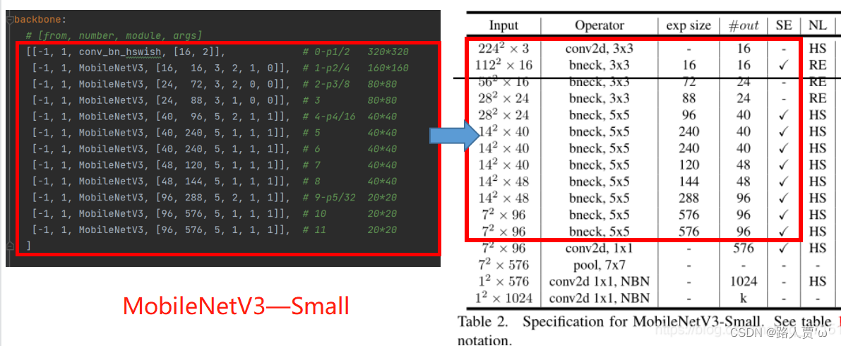
 然后运行yolo.py
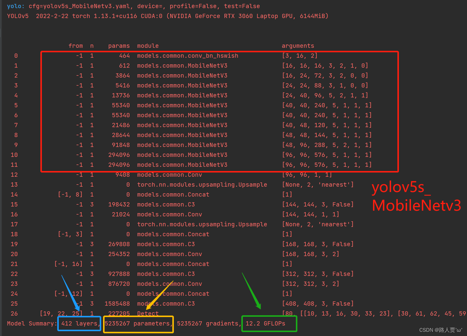


【本文地址】