| TensorFlow 处理图片 | 您所在的位置:网站首页 › sazabi什么意思 › TensorFlow 处理图片 |
TensorFlow 处理图片

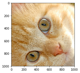
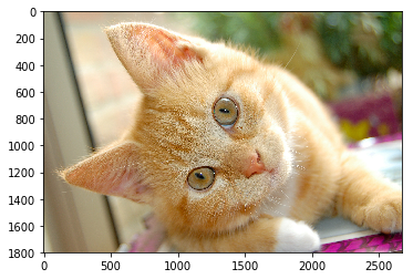
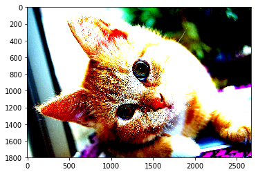
目标:介绍如何对图像数据进行预处理使训练得到的神经网络模型尽可能小地被无关因素所影响。但与此同时,复杂的预处理过程可能导致训练效率的下降。为了减少预处理对于训练速度的影响,TensorFlow 提供了多线程处理输入数据的解决方案。 TFRecord 输入数据格式TensorFlow 提供了一种统一的格式来存储数据(TFRecord)。TFRecord 文件中的数据都是通过 tf.train.Example Protocol Buffer 的格式存储的。 tf.train.Example的定义: message Example { Features features = 1; }; message Features { map feature = 1; }; message Features { oneof kind { BytesList bytes_list = 1; FloatList float_list = 2; Int64List int64_list = 3; } };train.Example 的数据结构比较简洁,包含了一个从属性名称到取值的字典。其中属性名称为一个字符串,属性的取值可以为字符串(BytesList),实数列表(FloatList)或者整数列表(Int64List)。 %pylab inline import tensorflow as tf import numpy as np from tensorflow.examples.tutorials.mnist import input_data Populating the interactive namespace from numpy and matplotlib def __int64__feature(value): '''生成整数型的属性''' return tf.train.Feature(int64_list= tf.train.Int64List(value=[value])) def __bytes__feature(value): '''生成字符型的属性''' return tf.train.Feature(bytes_list= tf.train.BytesList(value=[value])) mnist = input_data.read_data_sets('E:/datasets/mnist/data', dtype= tf.uint8, one_hot= True) Extracting E:/datasets/mnist/data\train-images-idx3-ubyte.gz Extracting E:/datasets/mnist/data\train-labels-idx1-ubyte.gz Extracting E:/datasets/mnist/data\t10k-images-idx3-ubyte.gz Extracting E:/datasets/mnist/data\t10k-labels-idx1-ubyte.gz images = mnist.train.images # 训练数据所对应的正确答案,可以作为一个属性保存在 TFRecord 中 labels = mnist.train.labels # 训练数据的图像分辨率,这可以作为 Example 中的一个属性 pixels = images.shape[1] num_examples = mnist.train.num_examples # 输出 TFRecord 文件的地址 filename = 'E:/datasets/mnist/output.tfrecords' # 创建一个 writer 来写 TFRecord 文件 writer = tf.python_io.TFRecordWriter(filename) for index in range(num_examples): # 将图片矩阵转化为一个字符串 image_raw = images[index].tostring() # 将一个样例转换为 Example Protocol Buffer,并将所有的信息写入到这个数据结构 examle = tf.train.Example(features = tf.train.Features(feature={ 'pixels': __int64__feature(pixels), 'label': __int64__feature(np.argmax(labels[index])), 'image_raw': __bytes__feature(image_raw) })) # 将一个 Example 写入 TFRecord 文件 writer.write(examle.SerializeToString()) writer.close()以上程序将 MNIST 数据集中所有的训练数据存储到一个 TFRecord 文件中。当数据量很大时,也可以将数据写入到多个 TFRecord 文件。 读取 TFRecord 文件中的数据 import tensorflow as tf # 创建一个 reader 来读取 TFRecord 文件中的样例 reader = tf.TFRecordReader() # 创建一个队列来维护输入文件列表 filename_queue = tf.train.string_input_producer(['E:/datasets/mnist/output.tfrecords']) # 从文件中读出一个样例。也可使用 read_up_to 函数一次性读取多个样例 _, serialized_example = reader.read(filename_queue) # 解析读入的一个样例。如果需要解析多个样例,可以用 parse_example 函数 features = tf.parse_single_example(serialized_example, features= { # TensorFlow 提供两种不同的属性解析方法。一种是 tf.FixedLenFeature,解析结果为一个 Tensor # 另一种方法为 tf.VarLenFeature,解析结果为 SparseTensor,用于处理稀疏数据 # 解析数据的格式需要和写入数据的格式一致 'image_raw': tf.FixedLenFeature([], tf.string), 'pixels': tf.FixedLenFeature([], tf.int64), 'label': tf.FixedLenFeature([], tf.int64), }) # tf.decode_raw 可以将字符串解析成图片对应的像素数组 images = tf.decode_raw(features['image_raw'], tf.uint8) labels = tf.cast(features['label'], tf.int32) pixels = tf.cast(features['pixels'], tf.int32) sess = tf.Session() # 启动多线程 coord = tf.train.Coordinator() threads = tf.train.start_queue_runners(sess= sess, coord= coord) # 每次运行可以读取 TFRecord 文件中的一个样例。当所有样例都读完之后,在此样例中程序会再重头读取 for i in range(10): image, label, pixel = sess.run([images, labels, pixels]) sess.close() INFO:tensorflow:Error reported to Coordinator: , Run call was cancelled INFO:tensorflow:Error reported to Coordinator: , Run call was cancelled 图像数据处理通过对图像的预处理,可以尽量避免模型受到无关因素的影响。在大部分图像识别问题中,通过图像预处理过程可以提高模型的准确率。 图像编码处理一张 RGB 色彩模式的图片可看作一个三维矩阵,矩阵的每一个数字表示图像上不同位置,不同颜色的亮度。然而图像在存储时并不是直接记录这些矩阵中的数字,而是记录经过压缩编码之后的结果。所要将一张图像还原成一个三维矩阵,需要解码的过程。TensorFlow 提供了对 jpeg 和 png 格式图像的编码/解码函数。 import matplotlib.pyplot as plt import tensorflow as tf import numpy as np # 读取图像的原始数据 image_raw_data = tf.gfile.FastGFile('E:/datasets/cat.jpg', 'rb').read() # 必须是 ‘rb’ 模式打开,否则会报错 with tf.Session() as sess: # 将图像使用 jpeg 的格式解码从而得到图像对应的三维矩阵 # tf.image.decode_jpeg 函数对 png 格式的图像进行解码。解码之后的结果为一个张量, ## 在使用它的取值之前需要明确调用运行的过程。 img_data = tf.image.decode_jpeg(image_raw_data) # 输出解码之后的三维矩阵。 print(img_data.eval()) [[[162 161 140] [162 162 138] [161 161 137] ..., [106 140 46] [101 137 47] [102 141 52]] [[164 162 139] [163 161 136] [163 161 138] ..., [104 138 43] [102 139 46] [108 138 50]] [[165 163 140] [165 163 138] [163 161 136] ..., [104 135 41] [102 137 43] [108 139 45]] ..., [[207 200 181] [206 199 180] [206 199 180] ..., [109 84 53] [107 84 53] [106 81 50]] [[205 200 180] [205 200 180] [206 199 180] ..., [106 83 49] [105 82 51] [106 81 50]] [[205 200 180] [205 198 179] [205 198 179] ..., [108 86 49] [105 82 48] [104 81 49]]] 打印图片 with tf.Session() as sess: plt.imshow(img_data.eval()) plt.show()
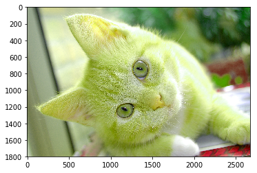
一般地,网上获取的图片的大小是不固定的,但是神经网络输入节点的个数是固定的。所以在将图像的像素作为输入提供给神经网络之前,需要将图片的大小统一。图片的大小调整有两种方式: 通过算法使得新的图片尽可能的保存原始图像上的所有信息。 Tensorflow 提供了四种不同的方法,并且将它们封装在 tf.image.resize_images 函数中。 裁剪或填充 保存完整信息 with tf.Session() as sess: resized = tf.image.resize_images(img_data, [300, 300], method=0) # TensorFlow的函数处理图片后存储的数据是float32格式的,需要转换成uint8才能正确打印图片。 print("Digital type: ", resized.dtype) print("Digital shape: ", resized.get_shape()) cat = np.asarray(resized.eval(), dtype='uint8') # tf.image.convert_image_dtype(rgb_image, tf.float32) plt.imshow(cat) plt.show() Digital type: Digital shape: (300, 300, 3)
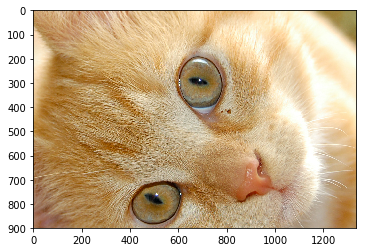
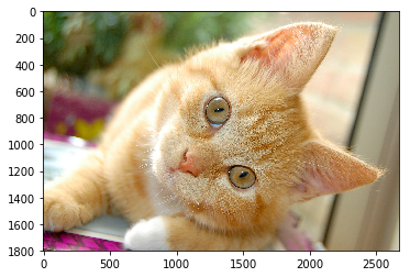
tf.image.resize_images 的 method 参数: Method 取值 图像大小调整算法 0 双线性插值法(Bilinear interpolation) 1 最近邻居法(Nearest neighbor interpolation) 2 双三次插值法(Bicubic interpolation) 3 面积插值法(Area interpolation) 裁剪和填充tf.image.resize_image_with_crop_or_pad 函数可以调整图像的大小。如果原始图像的尺寸大于目标图像这个函数会自动裁取原始图像中居中的部分;如果目标图像大于原始图像,这个函数会自动在原始图像的四周填充全 \(0\) 背景。 with tf.Session() as sess: croped = tf.image.resize_image_with_crop_or_pad(img_data, 1000, 1000) padded = tf.image.resize_image_with_crop_or_pad(img_data, 3000, 3000) plt.imshow(croped.eval()) plt.show() plt.imshow(padded.eval()) plt.show()
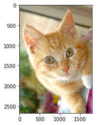
tf.image.central_crop 函数可以按比例裁剪图像。其中比例取值:\((0, 1]\) 的实数。 with tf.Session() as sess: central_cropped = tf.image.central_crop(img_data, 0.5) plt.imshow(central_cropped.eval()) plt.show()
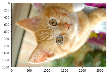
以上的函数都是截取或填充图像的中间部分。使用 tf.image.crop_to_bounding_box 和 tf.image.pad_to_bounding_box 函数可以裁剪或填充给定区域的图像。 翻转图片 with tf.Session() as sess: # 上下翻转 flipped1 = tf.image.flip_up_down(img_data) plt.imshow(flipped1.eval()) plt.show() # 左右翻转 flipped2 = tf.image.flip_left_right(img_data) plt.imshow(flipped2.eval()) plt.show() #对角线翻转 transposed = tf.image.transpose_image(img_data) plt.imshow(transposed.eval()) plt.show()
在很多图像识别问题中,图像的翻转不会影响识别结果。于是在训练图像识别的神经网络时,可以随机地翻转训练图像,这样训练得到的模型可以识别不同角度的实体。因而随机翻转训练图像是一种零成本的很常用的图像预处理方式。TensorFlow 提供了方便的 API 完成随机图像翻转的过程。以下代码实现了这个过程: with tf.Session() as sess: # 以一定概率上下翻转图片。 flipped = tf.image.random_flip_up_down(img_data) plt.imshow(flipped.eval()) plt.show() # 以一定概率左右翻转图片。 flipped = tf.image.random_flip_left_right(img_data) plt.imshow(flipped.eval()) plt.show()
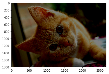
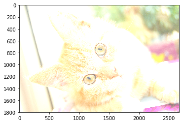
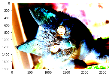
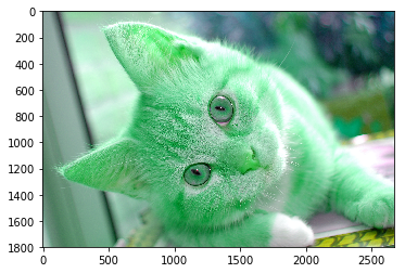
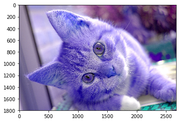
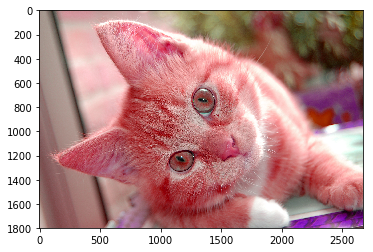
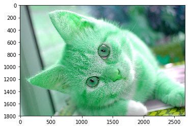
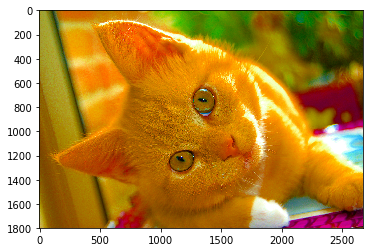
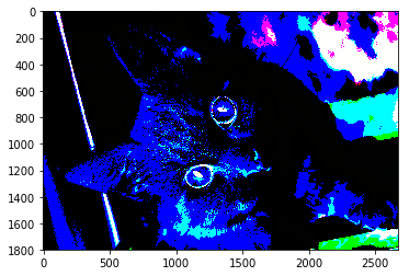
和图像翻转类似,调整图像的亮度、对比度、饱和度和色相在很多图像识别应用中都不会影响识别结果。所以在训练神经网络模型时,可以随机调整训练图像的这些属性,从而使训练得到的模型尽可能小的受到无关因素的影响。以下代码可以完成此功能: with tf.Session() as sess: # 将图片的亮度 -0.5。 adjusted = tf.image.adjust_brightness(img_data, -0.5) plt.imshow(adjusted.eval()) plt.show() # 将图片的亮度 +0.5 adjusted = tf.image.adjust_brightness(img_data, 0.5) plt.imshow(adjusted.eval()) plt.show() # 在[-max_delta, max_delta)的范围随机调整图片的亮度。 adjusted = tf.image.random_brightness(img_data, max_delta=0.5) plt.imshow(adjusted.eval()) plt.show()
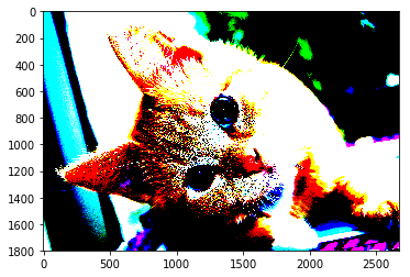
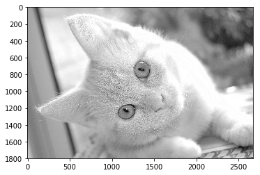
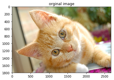
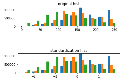
标准化处理可以使得不同的特征具有相同的尺度(Scale)。这样,在使用梯度下降法学习参数的时候,不同特征对参数的影响程度就一样了。tf.image.per_image_standardization(image),此函数的运算过程是将整幅图片标准化(不是归一化),加速神经网络的训练。主要有如下操作,\(\frac{x - mean}{adjusted\_stddev}\),其中\(x\)为图片的 RGB 三通道像素值,\(mean\)分别为三通道像素的均值,\(adjusted\_stddev = \max \left(stddev, \frac{1.0}{\sqrt{image.NumElements()}}\right)\)。 - \(stddev\)为三通道像素的标准差,image.NumElements()计算的是三通道各自的像素个数。 import tensorflow as tf import matplotlib.image as img import matplotlib.pyplot as plt import numpy as np sess = tf.InteractiveSession() image = img.imread('E:/datasets/cat.jpg') shape = tf.shape(image).eval() h,w = shape[0],shape[1] standardization_image = tf.image.per_image_standardization(image) #标准化 fig = plt.figure() fig1 = plt.figure() ax = fig.add_subplot(111) ax.set_title('orginal image') ax.imshow(image) ax1 = fig1.add_subplot(311) ax1.set_title('original hist') ax1.hist(sess.run(tf.reshape(image,[h*w,-1]))) ax1 = fig1.add_subplot(313) ax1.set_title('standardization hist') ax1.hist(sess.run(tf.reshape(standardization_image,[h*w,-1]))) plt.ion() plt.show()
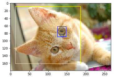
在很多图像识别数据集中,图像中需要关注的物体通常会被标注框圈出来。使用 tf.image.draw_bounding_boxes 函数便可以实现。 with tf.Session() as sess: # 将图像缩小一些,这样可视化能够让标注框更加清晰 img_data = tf.image.resize_images(img_data, [180, 267], method= 1) # tf.image.draw_bounding_boxes 函数要求图像矩阵中的数字为实数类型。 # tf.image.draw_bounding_boxes 函数的输入是一个 batch 的数据,也就是多张图像组成的四维矩阵,所以需要将解码后的图像加一维 batched = tf.expand_dims(tf.image.convert_image_dtype(img_data, tf.float32), 0) # 给出每张图像的所有标注框。一个标注框有四个数字,分别代表 [y_min, x_min, y_max, x_max] ## 注意这里给出的数字都是图像的相对位置。比如在 180 * 267 的图像中 [0.35, 0.47, 0.5, 0.56] 代表了从 (63, 125) 到 (90, 150) ### 的图像。 boxes = tf.constant([[[0.05, 0.05, 0.9, 0.7], [0.35, 0.47, 0.5, 0.56]]]) result = tf.image.draw_bounding_boxes(batched, boxes) plt.imshow(result[0].eval()) plt.show()
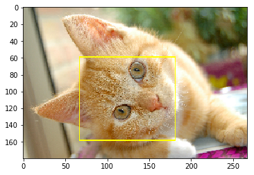
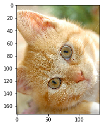
和随机翻转图像、随机调整颜色类似,随机截取图像上有信息含量的部分也是一个提高模型健壮性(robustness)的一种方式。这样可以使训练得到的模型不受被识别物体的大小的影响。tf.image.sample_distorted_bounding_box 函数可以完成随机截取图像的过程。 with tf.Session() as sess: boxes = tf.constant([[[0.05, 0.05, 0.9, 0.7], [0.35, 0.47, 0.5, 0.56]]]) # 可以通过提供随机标注框的方式来告诉随机截取图像的算法哪些部分是 “有信息量” 的。 begin, size, bbox_for_draw = tf.image.sample_distorted_bounding_box( tf.shape(img_data), bounding_boxes=boxes) # 通过标注框可视化随机截取得到的图像 batched = tf.expand_dims(tf.image.convert_image_dtype(img_data, tf.float32), 0) image_with_box = tf.image.draw_bounding_boxes(batched, bbox_for_draw) plt.imshow(image_with_box[0].eval()) plt.show() # 截取随机出来的图像,因为算法带有随机成分,所以每次的结果都可能不相同 distorted_image = tf.slice(img_data, begin, size) plt.imshow(distorted_image.eval()) plt.show()
|


【本文地址】