| MATLAB PDE工具箱简单教程 | 您所在的位置:网站首页 › pde导出 › MATLAB PDE工具箱简单教程 |
MATLAB PDE工具箱简单教程
|
PDE 即 Partial Differential Equations 因为用起来太懵了所以写下这篇博客 先说 Alt 菜单下面的一行按钮,分别是:以角点绘制矩形、中心点角点绘制矩形、直径画圆、半径画圆、折线绘制多边形边界模式、PDE 说明、初始化网格、细化网格、求解、绘制图像、缩放右边的下拉菜单是选择问题类型,因为许多物理学的方面都需要用到偏微分方程
下文按照这行按钮的顺序解释用法
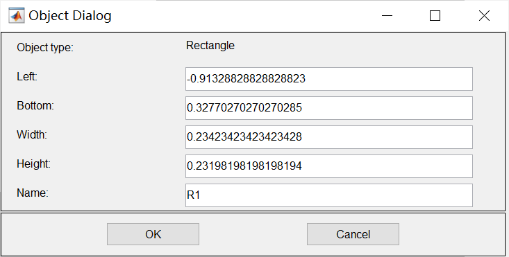
绘制图形一般是随意画一个然后双击该图形调整其位置,图形名字也可以改也可以在 Alt 菜单 Draw 下的对应指令 然后是边界模式,跟 Alt 菜单 Boundary 下的 Boundary Mode 是一样的设置边界条件一般是在边界模式下双击要设置条件的边界 之后是在区域内设置 PDE,我只能将它粗略翻译为“PDE 说明”设置各区域的 PDE 个人建议用 Alt 菜单 PDE 下的 PDE Mode,在该模式下可以对各个区域分别编辑设置 PDE切换到该模式之后双击各个图形区域即可 界面如上图与边界条件的界面相似,上边是等式形式,左边是方程类型,右边是参数及其描述由于通用类型下 MATLAB 没给出 Description,这里以 Heat Transfer 热传导类型为例 之后就是网格划分了,先说第二个网格细化,其实就是把求解前离散化的网格划分的更细,这样解也会更加精确根据使用需求选择合适的细化程度,但化的太细之后会严重增加计算负担,并且甚至会超出 MATLAB 的矩阵大小导致不能导出解(这种情况应该只能导出图像)值得一提的是在后面导出解的时候,导出的解是各个离散后点的位置上的数值解,所以如果要导出解的话一般来说都是要将离散化前后对应点的标号和坐标一并导出的导出离散化前后的对应关系在 Alt 菜单 Mesh 下的 Export Mesh 里,注意导出之前是需要先划分网格的(Mesh) 后面是求解,需要先在 Alt 菜单下 Parameters 里输入各种参数/条件,由于不同问题类型下的参数不同,这里不做赘述设置好参数/条件之后就可以求解了,求解之后可以导出解,解的矩阵对应列数是离散化后点的编号 最后是画图像,有3D有动图,也可以调整颜色,根据所需选择即可 附上一段代码: % This script is written and read by pdetool and should NOT be edited. % There are two recommended alternatives: % 1) Export the required variables from pdetool and create a MATLAB script % to perform operations on these. % 2) Define the problem completely using a MATLAB script. See % https://www.mathworks.com/help/pde/examples.html for examples % of this approach. clear; clc; [pde_fig,ax]=pdeinit; pdetool('appl_cb',9); set(ax,'DataAspectRatio',[1 142.85714285714286 1]); set(ax,'PlotBoxAspectRatio',[1.5000000000000004 1 142.85714285714286]); set(ax,'XLim',[-0.001 0.02]); set(ax,'YLim',[-0.5 1.5]); set(ax,'XTickMode','auto'); set(ax,'YTickMode','auto'); %additional thickness = 0.0207; second_pos = 0.0006 + thickness; third_pos = second_pos + 0.0036; fourth_pos = third_pos + 0.0055; %additional % Geometry description: pderect([0 0.0006 1 0],'R1'); pderect([0.0006 second_pos 1 0],'R2'); pderect([second_pos third_pos 1 0],'R3'); pderect([third_pos fourth_pos 1 0],'R4'); set(findobj(get(pde_fig,'Children'),'Tag','PDEEval'),'String','R1+R2+R3+R4'); % Boundary conditions: pdetool('changemode',0); pdesetbd(12,... 'dir',... 1,... '0',... '0'); pdesetbd(11,... 'dir',... 1,... '0',... '0'); pdesetbd(10,... 'dir',... 1,... '0',... '0'); pdesetbd(9,... 'dir',... 1,... '0',... '0'); pdesetbd(8,... 'dir',... 1,... '0',... '0'); pdesetbd(7,... 'dir',... 1,... '0',... '0'); pdesetbd(6,... 'dir',... 1,... '0',... '0'); pdesetbd(5,... 'dir',... 1,... '0',... '0'); pdesetbd(2,... 'neu',... 1,... '8.36',... '309.32'); pdesetbd(1,... 'dir',... 1,... '1',... '65'); % Mesh generation: setappdata(pde_fig,'Hgrad',1.3); setappdata(pde_fig,'refinemethod','regular'); setappdata(pde_fig,'jiggle',char('on','mean','')); setappdata(pde_fig,'MesherVersion','preR2013a'); pdetool('initmesh'); % PDE coefficients: pdeseteq(2,... '0.082!0.028!0.37!0.045',... '0!0!0!0',... '(1)+(0).*(65)!(0)+(0).*(37)!(0)+(0).*(30)!(0)+(0).*(37)',... '(300).*(1377)!(1.18).*(1005)!(862).*(2100)!(74.2).*(1726)',... '0:3600',... '37',... '0.0',... '[0 100]'); setappdata(pde_fig,'currparam',... ['300!1.18!862!74.2 ';... '1377!1005!2100!1726 ';... '0.082!0.028!0.37!0.045';... '1!0!0!0 ';... '0!0!0!0 ';... '65!37!37!37 ']); % Solve parameters: setappdata(pde_fig,'solveparam',... char('0','1260','10','pdeadworst',... '0.5','longest','0','1E-4','','fixed','Inf')); % Plotflags and user data strings: setappdata(pde_fig,'plotflags',[1 1 1 1 1 1 6 1 0 0 0 5401 1 0 0 0 0 1]); setappdata(pde_fig,'colstring',''); setappdata(pde_fig,'arrowstring',''); setappdata(pde_fig,'deformstring',''); setappdata(pde_fig,'heightstring',''); % Solve PDE: pdetool('solve'); pdetool('export', 5);
|
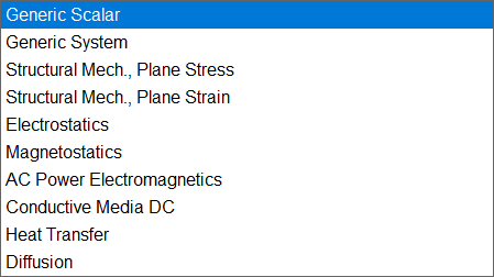 分别是:通用标量(?)、通用系统、结构力学:平面应力、结构力学:平面应变 静电学、静磁学、交流电源电磁学、直流导电介质、热传导、扩散选择这些主要是方便方程参数的输入和求解时一些条件的设定,选择所求解的问题类型,MATLAB 会把参数/条件的框提示改成相应的物理意义
 界面如图,上面是边界条件的等式形式,是提示参数对应系数的左边是条件类型,纽曼边界条件和狄利克雷边界条件右边的 Description 在上文中选择问题类型之后会给出各个方程系数的物理意义
【本文地址】