三维变换矩阵实战

2024-07-16 02:22| 来源: 网络整理| 查看: 265

一、旋转矩阵（右手坐标系）绕x轴旋转

旋转矩阵：右边矩阵是点云的原始坐标，左边的是旋转矩阵

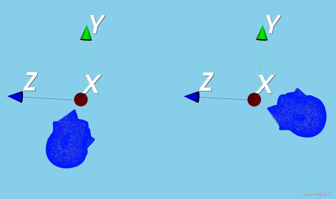
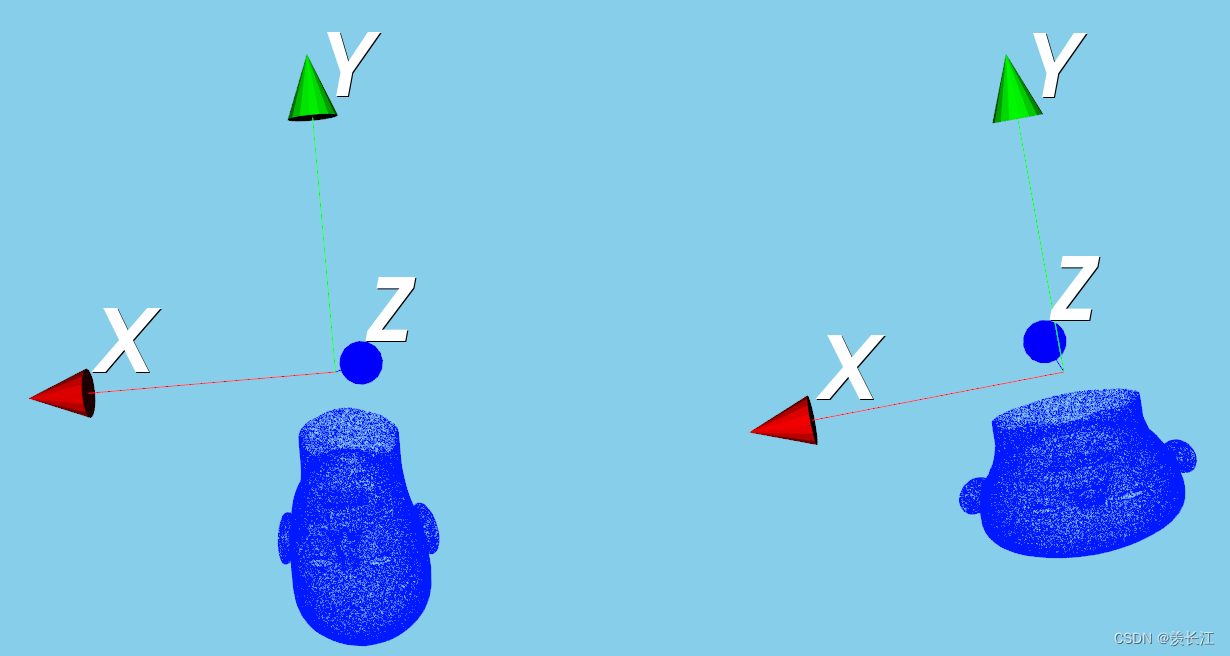
$\begin{bmatrix} 1&0 &0 \\ 0&cos\beta &-sin\beta \\ 0&sin\beta & cos\beta \end{bmatrix}$ $\begin{bmatrix} x\\ y \\z \end{bmatrix}$

可视化：绕x轴旋转90度

代码：

import vtk import numpy as np import math def pointPolydataCreate(pointCloud): points = vtk.vtkPoints() cells = vtk.vtkCellArray() i = 0 for point in pointCloud: points.InsertPoint(i, point[0], point[1], point[2]) cells.InsertNextCell(1) cells.InsertCellPoint(i) i += 1 PolyData = vtk.vtkPolyData() PolyData.SetPoints(points) PolyData.SetVerts(cells) mapper = vtk.vtkPolyDataMapper() mapper.SetInputData(PolyData) actor = vtk.vtkActor() actor.SetMapper(mapper) actor.GetProperty().SetColor(0.0, 0.1, 1.0) return actor def visiualize(pointCloud, pointCloud2): colors = vtk.vtkNamedColors() actor1 = pointPolydataCreate(pointCloud) actor2 = pointPolydataCreate(pointCloud2) Axes = vtk.vtkAxesActor() # 可视化 renderer1 = vtk.vtkRenderer() renderer1.SetViewport(0.0, 0.0, 0.5, 1) renderer1.AddActor(actor1) renderer1.AddActor(Axes) renderer1.SetBackground(colors.GetColor3d('skyblue')) renderer2 = vtk.vtkRenderer() renderer2.SetViewport(0.5, 0.0, 1.0, 1) renderer2.AddActor(actor2) renderer2.AddActor(Axes) renderer2.SetBackground(colors.GetColor3d('skyblue')) renderWindow = vtk.vtkRenderWindow() renderWindow.AddRenderer(renderer1) renderWindow.AddRenderer(renderer2) renderWindow.SetSize(1040, 880) renderWindow.Render() renderWindow.SetWindowName('PointCloud') renderWindowInteractor = vtk.vtkRenderWindowInteractor() renderWindowInteractor.SetRenderWindow(renderWindow) renderWindowInteractor.Initialize() renderWindowInteractor.Start() pointCloud = np.loadtxt("C:/Users/A/Desktop/pointCloudData/model.txt") #读取点云数据 angel_x = 90 # 旋转角度 radian = angel_x * np.pi / 180 # 旋转弧度 Rotation_Matrix_1 = [ # 绕x轴三维旋转矩阵 [1, 0, 0], [0, math.cos(radian), -math.sin(radian)], [0, math.sin(radian), math.cos(radian)]] Rotation_Matrix_1 = np.array(Rotation_Matrix_1) p = np.dot(Rotation_Matrix_1, pointCloud.T) # 计算 p = p.T visiualize(pointCloud, p) 绕y轴旋转

旋转矩阵：

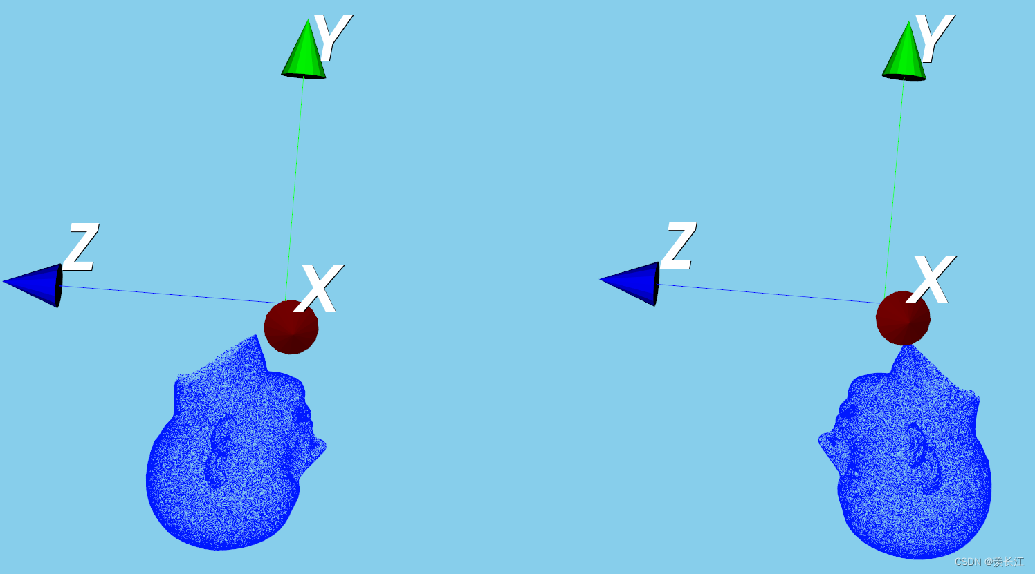
$\begin{bmatrix} cos\beta &0 &sin\beta \\ 0&1 &0 \\ -sin\beta &0 &cos\beta \end{bmatrix}$ $\begin{bmatrix} x\\ y \\z \end{bmatrix}$

可视化：绕y轴旋转180度

代码：

angel_y = 180 # 旋转角度 radian = angel_y * np.pi / 180 # 旋转弧度 Rotation_Matrix_2 = [ # 绕y轴三维旋转矩阵 [math.cos(radian), 0, math.sin(radian)], [0, 1, 0], [-math.sin(radian), 0, math.cos(radian)]] Rotation_Matrix_1 = np.array(Rotation_Matrix_1) p = np.dot(Rotation_Matrix_1, pointCloud.T) # 计算 p = p.T visiualize(pointCloud, p) 绕z轴旋转

旋转矩阵：

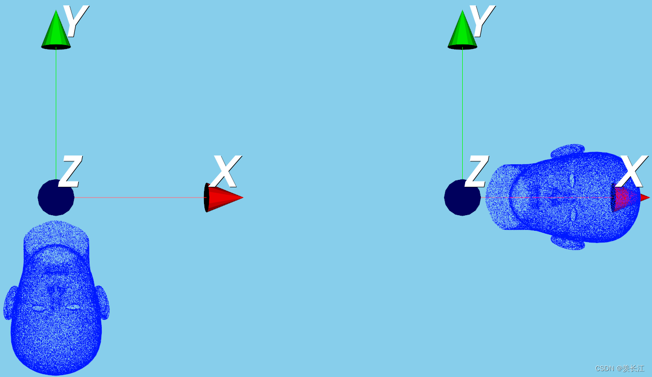
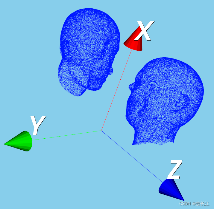
$\begin{bmatrix} cos\beta &-sin\beta &0 \\ sin\beta &cos\beta & 0\\ 0&0 & 1 \end{bmatrix}$ $\begin{bmatrix} x\\ y \\z \end{bmatrix}$

可视化：绕z轴旋转90度

代码：

angel_z = 90 # 旋转角度 radian = angel_z * np.pi / 180 # 旋转弧度 Rotation_Matrix_1 = [ # 绕z轴三维旋转矩阵 [math.cos(radian), -math.sin(radian), 0], [math.sin(radian), math.cos(radian), 0], [0, 0, 1]] Rotation_Matrix_1 = np.array(Rotation_Matrix_1) p = np.dot(Rotation_Matrix_1, pointCloud.T) # 计算 p = p.T visiualize(pointCloud, p) 线绕z轴旋转，再绕x轴旋转：

旋转矩阵: 线绕哪个轴转，xyz矩阵就和哪和轴的旋转矩阵先计算

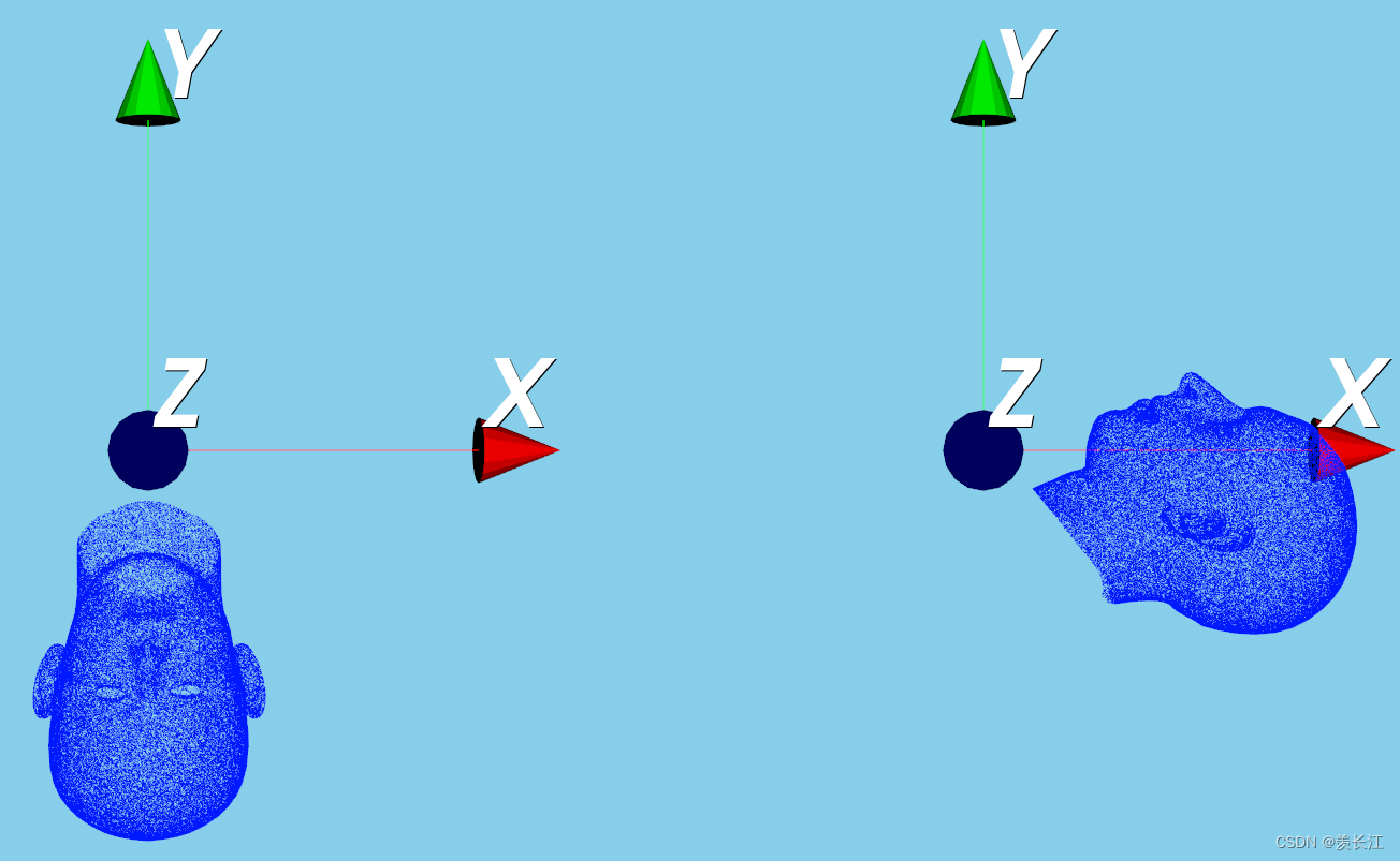
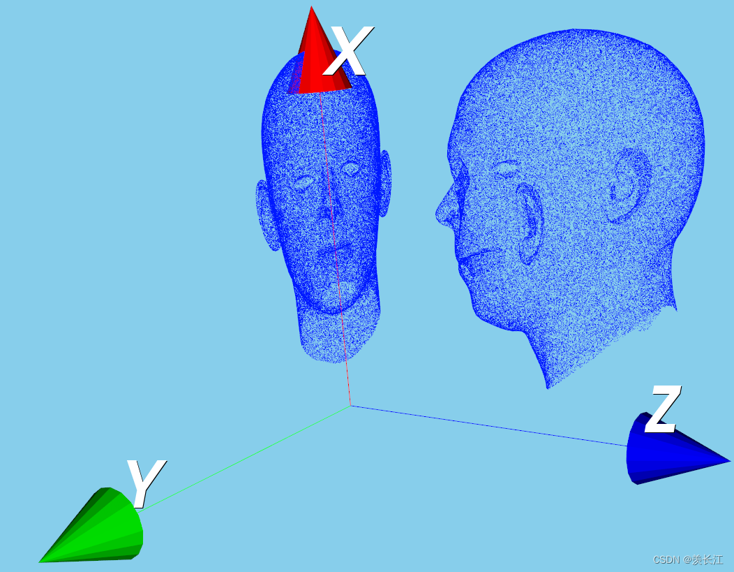
$\begin{bmatrix} 1&0 &0 \\ 0&cos\beta &-sin\beta \\ 0&sin\beta & cos\beta \end{bmatrix}$ $\begin{bmatrix} cos\beta &-sin\beta &0 \\ sin\beta &cos\beta & 0\\ 0&0 & 1 \end{bmatrix}$ $\begin{bmatrix} x\\ y \\z \end{bmatrix}$

可视化：先绕z轴旋转90度，再绕x轴旋转90度

代码：

angel_z = 90 # 旋转角度 radian = angel_z * np.pi / 180 # 旋转弧度 Rotation_Matrix_z = [ # 绕z轴三维旋转矩阵 [math.cos(radian), -math.sin(radian), 0], [math.sin(radian), math.cos(radian), 0], [0, 0, 1]] angel_x = 90 # 旋转角度 radian = angel_x * np.pi / 180 # 旋转弧度 Rotation_Matrix_x = [ # 绕x轴三维旋转矩阵 [1, 0, 0], [0, math.cos(radian), -math.sin(radian)], [0, math.sin(radian), math.cos(radian)]] Rotation_Matrix_z = np.array(Rotation_Matrix_z) Rotation_Matrix_x = np.array(Rotation_Matrix_x) p = np.dot(Rotation_Matrix_z, pointCloud.T) # 计算 p = np.dot(Rotation_Matrix_x, p) # 计算 p = p.T visiualize(pointCloud, p) 二、缩放矩阵

缩放矩阵：

$\begin{bmatrix} k_{x}&0 &0 \\ 0& k_{y} &0 \\ 0&0 &k_{z} \end{bmatrix}$

计算过程：三个k是xyz对应的缩放系数

$\begin{bmatrix} k_{x}&0 &0 \\ 0& k_{y} &0 \\ 0&0 &k_{z} \end{bmatrix}$ $\begin{bmatrix} x\\ y \\z \end{bmatrix}=$ $\begin{bmatrix} k_{x}x\\k_{y} y \\k_{z}z \end{bmatrix}$

x坐标变为原来的1.5倍，y变为0.7倍，z不变

$\begin{bmatrix} 1.5&0 &0 \\ 0& 0.7 &0 \\ 0&0 &1 \end{bmatrix}$ $\begin{bmatrix} x\\ y \\z \end{bmatrix}=$ $\begin{bmatrix} 1.5x\\0.7 y \\1z \end{bmatrix}$

可视化：

三、镜像矩阵

3D镜像矩阵：

$\begin{bmatrix} 1-2n_x{}^{2} & -2n_x{}n_{y} &-2n_x{}n_{z} \\ -2n_x{}n_{y} &1-2n_y{}^{2} &-2n_y{}n_{z} \\ -2n_x{}n_{z} &-2n_y{}n_{z} & 1-2n_z{}^{2} \end{bmatrix}$

$n=\begin{bmatrix} n_{x} &n_{y} & n_{z} \end{bmatrix}$

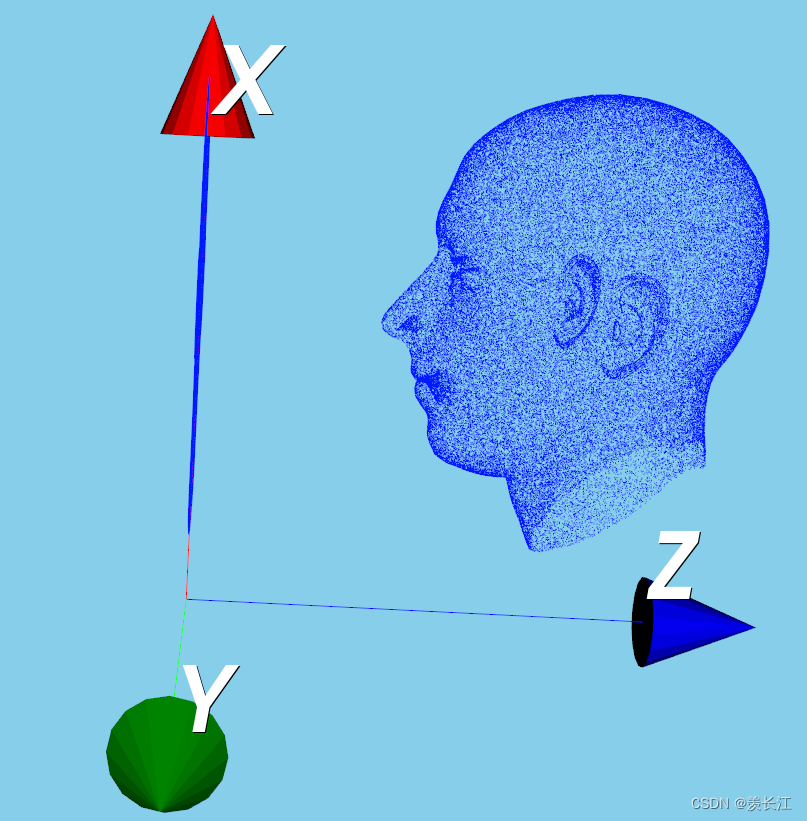
向量n是垂直于镜像平面的单位向量

三维点云对xz平面的镜像：

①首先，确定一个垂直于xz平面的单位向量 n=[0, 1, 0]

②将该单位向量带入上述3D镜像矩阵

可视化：

代码：

import vtk import numpy as np import math def pointPolydataCreate(pointCloud): points = vtk.vtkPoints() cells = vtk.vtkCellArray() i = 0 for point in pointCloud: points.InsertPoint(i, point[0], point[1], point[2]) cells.InsertNextCell(1) cells.InsertCellPoint(i) i += 1 PolyData = vtk.vtkPolyData() PolyData.SetPoints(points) PolyData.SetVerts(cells) mapper = vtk.vtkPolyDataMapper() mapper.SetInputData(PolyData) actor = vtk.vtkActor() actor.SetMapper(mapper) actor.GetProperty().SetColor(0.0, 0.1, 1.0) return actor def visiualize(pointCloud, pointCloud2): colors = vtk.vtkNamedColors() actor1 = pointPolydataCreate(pointCloud) actor2 = pointPolydataCreate(pointCloud2) Axes = vtk.vtkAxesActor() # 可视化 renderer1 = vtk.vtkRenderer() renderer1.SetViewport(0.0, 0.0, 0.5, 1) renderer1.AddActor(actor1) renderer1.AddActor(Axes) renderer1.SetBackground(colors.GetColor3d('skyblue')) renderer2 = vtk.vtkRenderer() renderer2.SetViewport(0.5, 0.0, 1.0, 1) renderer2.AddActor(actor1) renderer2.AddActor(actor2) renderer2.AddActor(Axes) renderer2.SetBackground(colors.GetColor3d('skyblue')) renderWindow = vtk.vtkRenderWindow() renderWindow.AddRenderer(renderer1) renderWindow.AddRenderer(renderer2) renderWindow.SetSize(1040, 880) renderWindow.Render() renderWindow.SetWindowName('PointCloud') renderWindowInteractor = vtk.vtkRenderWindowInteractor() renderWindowInteractor.SetRenderWindow(renderWindow) renderWindowInteractor.Initialize() renderWindowInteractor.Start() pointCloud = np.loadtxt("C:/Users/A/Desktop/pointCloudData/model.txt") #读取点云数据 nx = 0 ny = 0 nz = 1 n = [nx, ny, nz] # 垂直xy平面的单位向量 # 镜像矩阵 Mirror_Matrix = [ [1-2*nx**2, -2*nx*ny, -2*nx*nz], [-2*nx*ny, 1-2*ny**2, -2*ny*nz], [-2*nx*nz, -2*ny*nz, 1-2*nz**2]] Mirror_Matrix = np.array(Mirror_Matrix) p = np.dot(Mirror_Matrix, pointCloud.T) # 计算 p = p.T visiualize(pointCloud, p) 四、错切矩阵沿xy平面错切（z不变）

矩阵计算过程

$H_{xy}(s, t)=\begin{bmatrix} 1 &0 &s \\ 0&1 &t \\ 0&0 &1 \end{bmatrix}$ $\begin{bmatrix} 1 &0 &s \\ 0&1 &t \\ 0&0 &1 \end{bmatrix} \begin{bmatrix} x\\ y \\ z \end{bmatrix}=\begin{bmatrix} x+sz\\y+tz \\ z \end{bmatrix}$

沿xz平面错切（y不变）

矩阵计算过程

$H_{xz}(s, t)=\begin{bmatrix} 1 &0 &s \\ 0&1 &0 \\ 0&t &1 \end{bmatrix}$ $\begin{bmatrix} 1 &0 &s \\ 0&1 &0 \\ 0&t &1 \end{bmatrix} \begin{bmatrix} x\\ y \\ z \end{bmatrix}=\begin{bmatrix} x+sz\\y \\ z+ty \end{bmatrix}$

沿yz平面错切（x不变）

矩阵计算过程

$H_{yz}(s, t)=\begin{bmatrix} 1 &0 &0 \\ s&1 &0 \\ t&0 &1 \end{bmatrix}$ $\begin{bmatrix} 1 &0 &0 \\ s&1 &0 \\ t&0 &1 \end{bmatrix} \begin{bmatrix} x\\ y \\ z \end{bmatrix}=\begin{bmatrix} x\\y+sx \\ z+tx \end{bmatrix}$

可视化：沿yz平面错切

代码：

pointCloud = np.loadtxt("C:/Users/A/Desktop/pointCloudData/model.txt") #读取点云数据 s = 0.3 t = 0.3 # 沿yz平面错切矩阵 Shear_Matrix = [ [1, 0, 0], [s, 1, 0], [t, 0, 1]] Shear_Matrix = np.array(Shear_Matrix) p = np.dot(Shear_Matrix, pointCloud.T) # 计算 p = p.T visiualize(pointCloud, p) 五、正交投影正交投影矩阵（投影到三维空间任意平面）：

$\begin{bmatrix} 1-n_{x}^{2} &-n_{x}n_{y} &-n_{x}n_{z} \\ -n_{x}n_{y}&1-n_{y}^{2} &-n_{y}n_{z} \\ -n_{x}n_{z}&-n_{y}n_{z} & 1-n_{z}^{2} \end{bmatrix}$

$n=\begin{bmatrix} n_{x} &n_{y} & n_{z} \end{bmatrix}$

向量n是垂直于投影平面的单位向量

可视化：点云在xy平面上的正交投影

六、平移矩阵

平移矩阵需要利用齐次矩阵(4*4矩阵)，下面是一个平移矩阵

最右边一列是xyz的位移量

$\begin{bmatrix} 1 &0 &0 & \Delta x \\ 0&1 &0 &\Delta y \\ 0&0 &1 & \Delta z\\ 0&0 & 0 & 1 \end{bmatrix}$

计算过程：

$\begin{bmatrix} 1 &0 &0 & \Delta x \\ 0&1 &0 &\Delta y \\ 0&0 &1 & \Delta z\\ 0&0 & 0 & 1 \end{bmatrix}$ $\begin{bmatrix} x\\y \\z \\ 1 \end{bmatrix}=\begin{bmatrix} x+\Delta x\\ y+\Delta y \\ z+\Delta z \\ 1 \end{bmatrix}$

线性变换+平移：

增加的平移对原来的线性变换没影响，可以将前面介绍的变换矩阵和平移结合

例如：沿xy平面错切+平移

$\begin{bmatrix} 1&0 &s &\Delta x \\ 0&1 &t &\Delta y \\ 0&0 &1 &\Delta z \\ 0& 0& 0 & 1 \end{bmatrix}$

【本文地址】

公司简介

联系我们