Python时间序列分析3

2024-06-07 12:06| 来源: 网络整理| 查看: 265

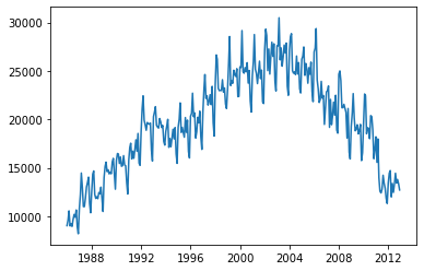
import pandas as pd import matplotlib.pyplot as plt import numpy as np from datetime import datetime,timedelta from time import time 数据读取与预处理 cat_fish = pd.read_csv('./data/catfish.csv',parse_dates=[0],index_col=0,squeeze=True) cat_fish.head() Date 1986-01-01 9034 1986-02-01 9596 1986-03-01 10558 1986-04-01 9002 1986-05-01 9239 Name: Total, dtype: int64 时序图 plt.plot(cat_fish) []

png

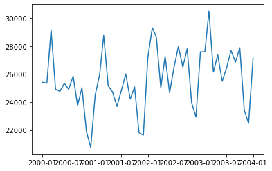
序列有明显的趋势性

start = datetime(2000,1,1) end = datetime(2004,1,1) plt.plot(cat_fish[start:end]) []

png

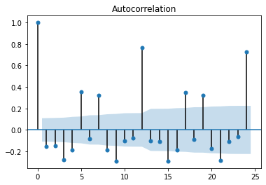
有很明显周期性

自相关系数图 from statsmodels.graphics.tsaplots import plot_acf,plot_pacf plot_acf(cat_fish.diff(1)[1:],lags=24)

png

偏自相关系数图 plot_pacf(cat_fish.diff(1)[1:])

png

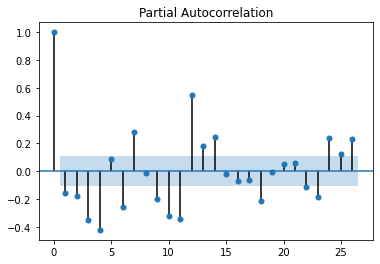
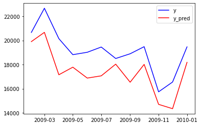
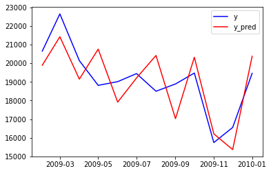
偏自相关系数图12步差分时，相关系数比较大，剔除趋势性后，原始数据还是呈现出明显的周期性

白噪声检验 from statsmodels.stats.diagnostic import acorr_ljungbox acorr_ljungbox(cat_fish.diff(1)[1:],lags=[6,12,18,24],return_df=True) lb_statlb_pvalue695.7197331.957855e-1812373.5414881.498233e-7218466.3003981.243989e-8724731.7566325.126647e-139

不是白噪声

使用SARIMA(0,1,0)x(1,0,1,12)进行预测

(0,1,0)是一阶差分，提取趋势性信息 (1,0,1,12)是ARMA(1,1),季节周期为12，提取季节性信息

模型训练 from statsmodels.tsa.statespace.sarimax import SARIMAX print(cat_fish.index[0],cat_fish.index[-1]) 1986-01-01 00:00:00 2012-12-01 00:00:00 train_end = datetime(2009,1,1) test_end = datetime(2010,1,1) train_data = cat_fish[:train_end] test_data = cat_fish[train_end + timedelta(days=1):test_end] model = SARIMAX(train_data,order=(0,1,0),seasonal_order=(1,0,1,12)) model_fit = model.fit() model_fit.summary() C:\Users\lipan\anaconda3\lib\site-packages\statsmodels\tsa\base\tsa_model.py:159: ValueWarning: No frequency information was provided, so inferred frequency MS will be used. warnings.warn('No frequency information was' C:\Users\lipan\anaconda3\lib\site-packages\statsmodels\tsa\base\tsa_model.py:159: ValueWarning: No frequency information was provided, so inferred frequency MS will be used. warnings.warn('No frequency information was' SARIMAX Results Dep. Variable:Total No. Observations: 277Model:SARIMAX(0, 1, 0)x(1, 0, [1], 12) Log Likelihood -2296.563Date:Sat, 03 Apr 2021 AIC 4599.126Time:17:13:59 BIC 4609.988Sample:01-01-1986 HQIC 4603.485- 01-01-2009 Covariance Type:opg coefstd errzP>|z|[0.0250.975]ar.S.L12 0.9889 0.007 135.425 0.000 0.975 1.003ma.S.L12 -0.7923 0.054 -14.692 0.000 -0.898 -0.687sigma2 9.069e+05 7.77e+04 11.666 0.000 7.55e+05 1.06e+06 Ljung-Box (Q):71.38 Jarque-Bera (JB): 0.57Prob(Q):0.00 Prob(JB): 0.75Heteroskedasticity (H):2.47 Skew: 0.08Prob(H) (two-sided):0.00 Kurtosis: 3.16 Warnings: [1] Covariance matrix calculated using the outer product of gradients (complex-step). 预测 predictions = model_fit.forecast(len(test_data)) predictions = pd.Series(predictions,index=test_data.index) residuals = test_data - predictions plt.plot(test_data,color ='b',label = 'y') plt.plot(predictions,color='r',label='y_pred') plt.legend() plt.show()

png

残差图 plt.plot(residuals) []

png

残差白噪声检验 acorr_ljungbox(residuals,lags=10,return_df=True) lb_statlb_pvalue12.9746430.08457923.7020850.15707339.9387640.019094416.4417910.002480516.6078130.005307617.9068280.006469721.1493840.003555821.9963740.004923922.0677070.0086671022.7895880.011550 循环预测 predictions_new = test_data.copy() for train_end in test_data.index: train_data = cat_fish[:train_end-timedelta(days = 1)] model = model = SARIMAX(train_data,order=(0,1,0),seasonal_order=(1,0,1,12),freq='MS') model_fit = model.fit() pred = model_fit.forecast(1) predictions_new[train_end] = pred plt.plot(test_data,color ='b',label = 'y') plt.plot(predictions_new,color='r',label='y_pred') plt.legend() plt.show()

png

plt.plot(test_data-predictions_new) []

png

print('RMSE:', np.sqrt(np.mean(residuals**2))) RMSE: 1832.9537663585463 residuals_new = test_data-predictions_new print('RMSE:', np.sqrt(np.mean(residuals_new**2))) RMSE: 1242.0409950292837

【本文地址】

公司简介

联系我们