| R语言实现NDVI的Sen | 您所在的位置:网站首页 › arcgis趋势分析结果 › R语言实现NDVI的Sen |
R语言实现NDVI的Sen
|
这几天在忙着把ArcGIS课程论文转换成大创项目,在这里记录一些过程和代码以便自己以后复盘和使用~参考了下面两篇博客的代码和绘图思路,使用R语言完成对NDVI的Sen-MK趋势分析和制图(使用的NDVI数据使用Python的ee和geemap实现): 1.从GEE获取2000-2018年的NDVI数据这一步只分享代码,不做解释(有想让笔者分享python版ee和geenap的可以咨询和私信呀) import ee import geemap geemap.set_proxy(port=7890)# 设置全局网络代理 Map = geemap.Map() # 指定所需数据范围 region = ee.Geometry.BBox(103.98254, 33.70393, 110.27061, 37.40193) def get_mean_ndvi(year): y1,y2 = f'{year}-01-01', f'{year+1}-01-01' ndvi_collection = (ee.ImageCollection('MODIS/MCD43A4_006_NDVI') .filterDate(y1,y2) .filterBounds(region)) ndvi = ndvi_collection.reduce(ee.Reducer.mean()) geemap.ee_export_image_to_drive( ndvi, description=f'ndvi{year}', folder='image',scale=1000,region=region) for y in range(2000,2019): get_mean_ndvi(y)2.Sen-MK趋势检验2.1导入将趋势检验中将使用的R包library(terra) library(trend) library(dplyr)2.2 读取长时间序列的NDVI数据并按研究区裁切list.files('./data/image/temporal-dataset/ndvi/',pattern = ".tif$") %>% paste0('./data/image/temporal-dataset/ndvi/',.)-> tif.file # 按研究区裁切栅格 weihe = vect('./data/渭河流域边界/') for (t in tif.file){ crop(rast(t),weihe,mask=T) |> writeRaster(t,overwrite=T) }2.3 定义Sen-MK趋势检验函数# Sen+MK计算 rast(tif.file)@ptr[['names']] |> length() -> times #用于时间序列MK趋势检验的时间跨度 print(times) fun_sen 2.5 计算的结果写出为tif# 输出结果 writeRaster(ndvi_sen, filename = "./data/image/temporal-dataset/ndvi_sen.tif", names=ndvi_sen@ptr[["names"]])3.结合slope值和Z统计量划分NDVI变化趋势3.1 对slope值重分类 ndvi.sen = rast('./data/image/temporal-dataset/ndvi_sen.tif')
# 取出最大和最小slope值
ndvi.sen$`sen-slope`|>
as.matrix() |>
na.omit() |>
max() -> max.slope
ndvi.sen$`sen-slope`|>
as.matrix() |>
na.omit() |>
min() -> min.slope
# slope new.slope ndvi.sen = rast('./data/image/temporal-dataset/ndvi_sen.tif')
# 取出最大和最小slope值
ndvi.sen$`sen-slope`|>
as.matrix() |>
na.omit() |>
max() -> max.slope
ndvi.sen$`sen-slope`|>
as.matrix() |>
na.omit() |>
min() -> min.slope
# slope new.slope 3.2 对Z统计值重分类 3.2 对Z统计值重分类 # 取出最大和最小Z值
ndvi.sen$`z-statistic`|>
as.matrix() |>
na.omit() |>
max() -> max.z
ndvi.sen$`z-statistic`|>
as.matrix() |>
na.omit() |>
min() -> min.z
# 对Z值进行重分类,确定显著性
# # |Z| = 1.96 通过95%置信度检验,显著
ndvi.sen$`z-statistic` %>%
classify(.,rbind(c(min.z,-1.96,2),
c(1.96,max.z,2),
c(-1.96,1.96,1)),
include.lowest=T) -> new.z # 取出最大和最小Z值
ndvi.sen$`z-statistic`|>
as.matrix() |>
na.omit() |>
max() -> max.z
ndvi.sen$`z-statistic`|>
as.matrix() |>
na.omit() |>
min() -> min.z
# 对Z值进行重分类,确定显著性
# # |Z| = 1.96 通过95%置信度检验,显著
ndvi.sen$`z-statistic` %>%
classify(.,rbind(c(min.z,-1.96,2),
c(1.96,max.z,2),
c(-1.96,1.96,1)),
include.lowest=T) -> new.z 3.3将Slope和Z值计算结果相乘,最后得到趋势变化划分# 将Slope和Z值计算结果相乘,最后得到趋势变化划分
ndvi.trend = new.z * new.slope
plot(ndvi.trend)
# ndvi.trend值含义:
# -2严重退化
# -1轻微退化
# 0稳定不变
# 1轻微改善
# 2明显改善 3.3将Slope和Z值计算结果相乘,最后得到趋势变化划分# 将Slope和Z值计算结果相乘,最后得到趋势变化划分
ndvi.trend = new.z * new.slope
plot(ndvi.trend)
# ndvi.trend值含义:
# -2严重退化
# -1轻微退化
# 0稳定不变
# 1轻微改善
# 2明显改善 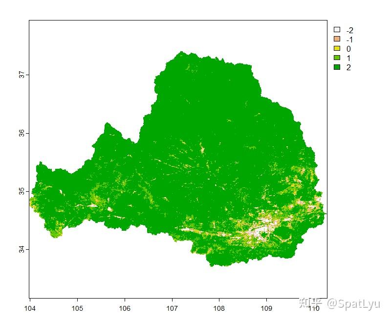 3.4将结果保存为栅格数据# 输出结果栅格
writeRaster(ndvi.trend,'./data/image/temporal-dataset/ndvi_trend.tif')4.制图并输出# 制图输出
library(tmap)
library(sf)
library(stars)
weihe = read_sf('./data/渭河流域边界/')
city = read_sf('./data/省市县-湖泊/渭河流域地级市region.shp')
citypoint = read_sf('./data/省市县-湖泊/地级市渭河流域_point.shp')
# ndvi.trend = read_stars('./data/image/temporal-dataset/ndvi_trend.tif')
# 设置主题
tmap_style('white')
# 绘图
tm_shape(ndvi.trend,bbox = c(103.8,33.65,110.4,37.45)) +
tm_raster(style='cat',
n=5,
labels = c('严重退化','轻微退化',
'稳定不变','轻微改善',
'明显改善'),
palette = c('#d7191c',
'#fdae61',
'#ffffbf',
'#abdda4',
'#2b83ba'),
title = "NDVI变化趋势",
midpoint = NA,
legend.reverse = T)+
tm_shape(weihe) +
tm_borders() +
tm_shape(city)+
tm_borders(lwd=0.7) +
tm_shape(citypoint) +
tm_dots(size=0.1,shape = 20) +
tm_text("NAME",just=c("left", "bottom")) +
tm_compass(type = 'arrow',
position = c("right", "top")) +
tm_scale_bar(position = c(0.1,0.03),
lwd = 1.5,text.size = 0.8) +
tm_add_legend(title="地级市边界",type='fill',col='grey',
size=0.3) +
tm_add_legend(type = "symbol", col = "black",
title = "地级市") +
tm_layout(legend.stack = 'horizontal',
legend.position = c(0.1,0.73),
main.title.position = 'center',
fontfamily = "serif") -> fig
tmap_save(fig,'./figure/NDVI_trend.png',dpi=600) 3.4将结果保存为栅格数据# 输出结果栅格
writeRaster(ndvi.trend,'./data/image/temporal-dataset/ndvi_trend.tif')4.制图并输出# 制图输出
library(tmap)
library(sf)
library(stars)
weihe = read_sf('./data/渭河流域边界/')
city = read_sf('./data/省市县-湖泊/渭河流域地级市region.shp')
citypoint = read_sf('./data/省市县-湖泊/地级市渭河流域_point.shp')
# ndvi.trend = read_stars('./data/image/temporal-dataset/ndvi_trend.tif')
# 设置主题
tmap_style('white')
# 绘图
tm_shape(ndvi.trend,bbox = c(103.8,33.65,110.4,37.45)) +
tm_raster(style='cat',
n=5,
labels = c('严重退化','轻微退化',
'稳定不变','轻微改善',
'明显改善'),
palette = c('#d7191c',
'#fdae61',
'#ffffbf',
'#abdda4',
'#2b83ba'),
title = "NDVI变化趋势",
midpoint = NA,
legend.reverse = T)+
tm_shape(weihe) +
tm_borders() +
tm_shape(city)+
tm_borders(lwd=0.7) +
tm_shape(citypoint) +
tm_dots(size=0.1,shape = 20) +
tm_text("NAME",just=c("left", "bottom")) +
tm_compass(type = 'arrow',
position = c("right", "top")) +
tm_scale_bar(position = c(0.1,0.03),
lwd = 1.5,text.size = 0.8) +
tm_add_legend(title="地级市边界",type='fill',col='grey',
size=0.3) +
tm_add_legend(type = "symbol", col = "black",
title = "地级市") +
tm_layout(legend.stack = 'horizontal',
legend.position = c(0.1,0.73),
main.title.position = 'center',
fontfamily = "serif") -> fig
tmap_save(fig,'./figure/NDVI_trend.png',dpi=600)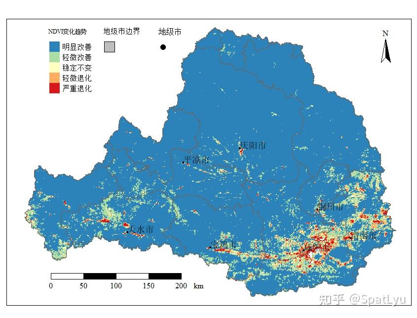 使用的总的代码如下: library(terra) library(trend) library(dplyr) list.files('./data/image/temporal-dataset/ndvi/',pattern = ".tif$") %>% paste0('./data/image/temporal-dataset/ndvi/',.)-> tif.file # 按研究区裁切栅格 weihe = vect('./data/渭河流域边界/') for (t in tif.file){ crop(rast(t),weihe,mask=T) |> writeRaster(t,overwrite=T) } # Sen+MK计算 rast(tif.file)@ptr[['names']] |> length() -> times #用于时间序列MK趋势检验的时间跨度 print(times) fun_sen as.matrix() |> na.omit() |> min() -> min.slope # slope new.slope # 取出最大和最小Z值 ndvi.sen$`z-statistic`|> as.matrix() |> na.omit() |> max() -> max.z ndvi.sen$`z-statistic`|> as.matrix() |> na.omit() |> min() -> min.z # 对Z值进行重分类,确定显著性 # # |Z| = 1.96 通过95%置信度检验,显著 ndvi.sen$`z-statistic` %>% classify(.,rbind(c(min.z,-1.96,2), c(1.96,max.z,2), c(-1.96,1.96,1)), include.lowest=T) -> new.z # 将Slope和Z值计算结果相乘,最后得到趋势变化划分 ndvi.trend = new.z * new.slope plot(ndvi.trend) # ndvi.trend值含义: # -2严重退化 # -1轻微退化 # 0稳定不变 # 1轻微改善 # 2明显改善 # 输出结果栅格 writeRaster(ndvi.trend,'./data/image/temporal-dataset/ndvi_trend.tif') # 制图输出 library(tmap) library(sf) library(stars) weihe = read_sf('./data/渭河流域边界/') city = read_sf('./data/省市县-湖泊/渭河流域地级市region.shp') citypoint = read_sf('./data/省市县-湖泊/地级市渭河流域_point.shp') # ndvi.trend = read_stars('./data/image/temporal-dataset/ndvi_trend.tif') # 设置主题 tmap_style('white') # 绘图 tm_shape(ndvi.trend,bbox = c(103.8,33.65,110.4,37.45)) + tm_raster(style='cat', n=5, labels = c('严重退化','轻微退化', '稳定不变','轻微改善', '明显改善'), palette = c('#d7191c', '#fdae61', '#ffffbf', '#abdda4', '#2b83ba'), title = "NDVI变化趋势", midpoint = NA, legend.reverse = T)+ tm_shape(weihe) + tm_borders() + tm_shape(city)+ tm_borders(lwd=0.7) + tm_shape(citypoint) + tm_dots(size=0.1,shape = 20) + tm_text("NAME",just=c("left", "bottom")) + tm_compass(type = 'arrow', position = c("right", "top")) + tm_scale_bar(position = c(0.1,0.03), lwd = 1.5,text.size = 0.8) + tm_add_legend(title="地级市边界",type='fill',col='grey', size=0.3) + tm_add_legend(type = "symbol", col = "black", title = "地级市") + tm_layout(legend.stack = 'horizontal', legend.position = c(0.1,0.73), main.title.position = 'center', fontfamily = "serif") -> fig tmap_save(fig,'./figure/NDVI_trend.png',dpi=600)完结收工! |
【本文地址】
公司简介
联系我们