| 【计算机视觉】计算机视觉的简单入门代码介绍(含源代码) | 您所在的位置:网站首页 › 3d打印入门教程图片 › 【计算机视觉】计算机视觉的简单入门代码介绍(含源代码) |
【计算机视觉】计算机视觉的简单入门代码介绍(含源代码)
|
文章目录
一、介绍二、项目代码2.1 导入三方包2.2 读取和展示图片2.3 在图像上绘画2.4 混合图像2.5 图像变换2.6 图像处理2.7 特征检测
一、介绍
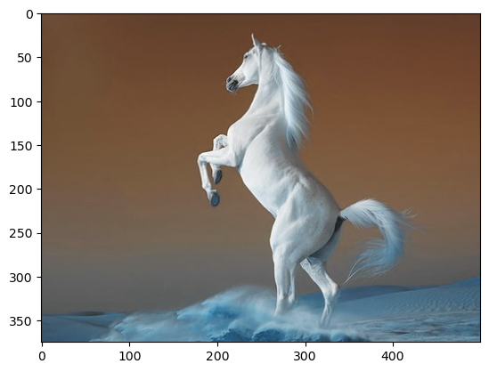
计算机视觉是一门研究计算机如何理解和解释图像和视频的学科。 它的目标是让计算机能够模拟人类视觉系统,让它们能够识别、分析和理解视觉输入。 计算机视觉利用计算机算法和技术来处理图像和视频数据。 这些算法可以从图像和视频中提取特征、识别和分类对象、检测和跟踪运动、测量和估计对象属性,以及生成和处理图像和视频。 计算机视觉的基本步骤包括图像采集、预处理、特征提取、目标检测和识别、图像分割和理解。 图像采集阶段涉及使用相机或其他图像采集设备采集图像或视频数据。 预处理阶段包括图像去噪、增强和调整,为进一步处理做好准备。 特征提取阶段涉及从图像中提取有意义的信息,例如边缘、角或纹理。 对象检测和识别涉及识别图像中的特定对象或场景,通常使用机器学习和深度学习算法来完成。 图像分割阶段将图像划分为不同的区域或对象,以供进一步分析和理解。 计算机视觉在各个领域都有应用,包括医学图像分析、自动驾驶、监控、面部识别、图像搜索和检索、增强现实等。 随着深度学习和神经网络的进步,计算机视觉在图像分类、目标检测和语义分割等任务中取得了重大突破。 尽管计算机视觉取得了许多进步,但它仍然面临复杂场景中的物体识别、图像理解、视觉推理和对抗性攻击等挑战。 未来,计算机视觉有望进一步发展和推动人工智能和计算机技术在视觉理解和感知方面的应用。 二、项目代码 2.1 导入三方包 import numpy as np import cv2 as cv import matplotlib.pyplot as plt 2.2 读取和展示图片 img = cv.imread('/kaggle/input/images-for-computer-vision/horse.jpg') plt.imshow(img)
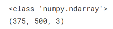
OpenCV 默认读取图像为 ‘BGR’,因此我们必须在打印前将图像转换为 ‘RGB’。 img_convert = cv.cvtColor(img, cv.COLOR_BGR2RGB) plt.imshow(img_convert)
使用 OpenCV,您可以在图像上绘制矩形、圆形或任何其他您想要的形状。 img = cv.imread('/kaggle/input/images-for-computer-vision/tiger1.jpg') # Rectangle # Color of the rectangle color = (240,150,240) ## For filled rectangle, use thickness = -1 cv.rectangle(img, (100,100),(300,300),color,thickness=10, lineType=8) ## (100,100) are (x,y) coordinates for the top left point of the rectangle and (300, 300) are (x,y) cordinates for the bottom righeight point # Circle color=(150,260,50) cv.circle(img, (650,350),100, color,thickness = 10) ## For filled circle, use thickness = -1 ## (250, 250) are (x,y) coordinates for the center of the circle and 100 is the radius # Text color=(50,200,100) font=cv.FONT_HERSHEY_SCRIPT_COMPLEX cv.putText(img, 'Save Tigers',(200,150), font, 5, color,thickness=5, lineType=20) # Converting BGR to RGB img_convert=cv.cvtColor(img, cv.COLOR_BGR2RGB) plt.imshow(img_convert)
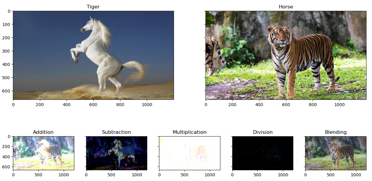
混合图像是指通过组合两个或多个图像,并结合原始图像的某些特征或信息来创建新图像。 这种合成可以通过简单的像素级操作或更复杂的图像处理技术来实现。 混合图像背后的核心思想是将两个图像的像素值组合起来生成一个新图像。 通常,这涉及对两幅图像的像素值进行加权平均,其中每个像素的权重决定了它对最终图像的贡献。 通过调整像素值的权重,可以控制每个原始图像在混合图像中的可见性。 除了简单的像素级混合,还有更高级的混合技术,可以实现更复杂的效果。 例如,混合图像可以利用图像融合、图像合成、多层混合等技术实现精细的控制和效果。 这些技术允许从不同图像中选择性地合成特定部分或特征,从而创建具有新颖视觉效果的图像。 混合图像在计算机图形学、图像处理和计算机视觉中有着广泛的应用。 它们可用于艺术创作、图像编辑、广告设计、数字娱乐以及模拟和增强现实。 混合图像还广泛用于特效、图像混合、风格转换和人脸合成等应用中。 总之,混合图像是一种通过合成多个图像来创建新图像的技术。 它通过像素级操作或先进的图像处理技术,将不同图像的特征和信息结合起来,产生具有独特视觉效果的图像。 def myplot(images, titles): fig, axs = plt.subplots(1, len(images), sharey = True) fig.set_figwidth(15) for img, ax, title in zip(images, axs, titles): if img.shape[-1] == 3: img = cv.cvtColor(img, cv.COLOR_BGR2RGB) else: img = cv.cvtColor(img, cv.COLOR_GRAY2BGR) ax.imshow(img) ax.set_title(title) img1 = cv.imread('/kaggle/input/images-for-computer-vision/horse.jpg') img2 = cv.imread('/kaggle/input/images-for-computer-vision/tiger1.jpg') # Resizing the img1 img1_resize = cv.resize(img1, (img2.shape[1], img2.shape[0])) # Adding, Subtracting, Multiplying and Dividing Images img_add = cv.add(img1_resize, img2) img_subtract = cv.subtract(img1_resize, img2) img_multiply = cv.multiply(img1_resize, img2) img_divide = cv.divide(img1_resize, img2) # Blending Images img_blend = cv.addWeighted(img1_resize, 0.3, img2, 0.7, 0) myplot([img1_resize, img2], ['Tiger','Horse']) myplot([img_add, img_subtract, img_multiply, img_divide, img_blend], ['Addition', 'Subtraction', 'Multiplication', 'Division', 'Blending'])
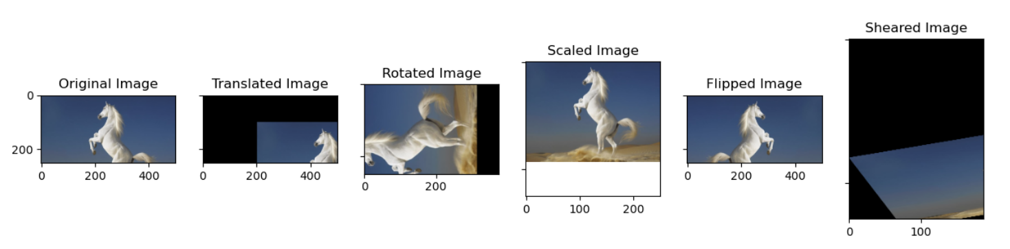
图像变换是指通过应用各种数学运算或技术来改变图像的外观或特征的过程。 图像变换的目标是以增强视觉质量、提取特定信息或实现所需视觉效果的方式处理图像。 img = cv.imread('/kaggle/input/images-for-computer-vision/horse.jpg') width, height, _ = img.shape # Translating M_translate = np.float32([[1, 0, 200],[0, 1, 100]]) # 200=> Translation along x-axis and 100=>translation along y-axis img_translate = cv.warpAffine(img, M_translate, (height, width)) # Rotating center = (width / 2, height / 2) M_rotate = cv.getRotationMatrix2D(center, angle = 90, scale = 1) img_rotate = cv.warpAffine(img, M_rotate, (width, height)) # Scaling scale_percent = 50 width = int(img.shape[1] * scale_percent / 100) height = int(img.shape[0] * scale_percent / 100) dim = (width, height) img_scale = cv.resize(img, dim, interpolation = cv.INTER_AREA) # Flipping img_flip=cv.flip(img,1) # 0:Along horizontal axis, 1:Along verticle axis, -1: first along verticle then horizontal # Shearing srcTri = np.array( [[0, 0], [img.shape[1] - 1, 0], [0, img.shape[0] - 1]] ).astype(np.float32) dstTri = np.array( [[0, img.shape[1] * 0.33], [img.shape[1] * 0.85, img.shape[0] * 0.25], [img.shape[1] * 0.15, img.shape[0] * 0.7]] ).astype(np.float32) warp_mat = cv.getAffineTransform(srcTri, dstTri) img_warp = cv.warpAffine(img, warp_mat, (height, width)) myplot([img, img_translate, img_rotate, img_scale, img_flip, img_warp], ['Original Image', 'Translated Image', 'Rotated Image', 'Scaled Image', 'Flipped Image', 'Sheared Image'])
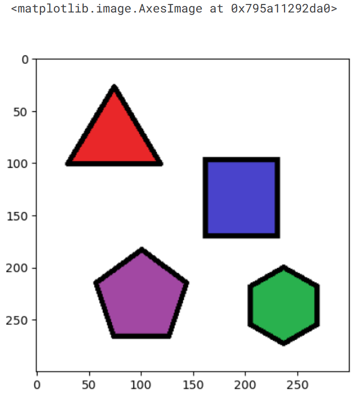
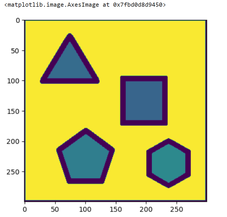
图像处理是指使用各种技术和算法对数字图像进行处理和分析。 它涉及对图像应用数学运算以提高图像质量、提取有用信息或执行特定任务。 可以在灰度、彩色或多光谱等不同域中对 2D 图像或 3D 体积执行图像处理。 图像处理有两大类:模拟和数字。 模拟图像处理涉及使用过滤、裁剪和调整曝光等技术处理物理照片或印刷品。 另一方面,数字图像处理涉及使用计算机算法以数字格式处理图像。 数字图像处理包含范围广泛的操作和技术,包括: 图像增强:通过对比度调整、亮度校正、降噪、锐化等技术来提高图像的视觉质量。图像恢复:图像恢复技术旨在恢复因噪声、模糊或压缩伪影等因素而退化的图像。图像压缩:压缩技术可减少图像数据的大小,同时保留重要的视觉信息。 无损和有损压缩算法用于图像的高效存储和传输。图像分割:图像分割涉及将图像划分为有意义的区域或对象。 它用于目标检测、图像理解和计算机视觉应用等任务。特征提取:特征提取技术从图像中识别和提取特定的模式或特征。 这些特征可用于对象识别、图像分类和图像检索等任务。图像配准:图像配准技术对齐同一场景的两个或多个图像以进行比较、融合或分析。 它在医学成像、遥感和计算机图形学等应用中很有用。对象检测和跟踪:边缘检测、轮廓分析和模板匹配等技术用于检测和跟踪图像或视频中的对象。图像分析:图像分析涉及从图像中提取定量信息,例如测量对象属性、计算图像统计数据或执行模式识别。图像处理在各个领域都有应用,包括医学成像、监控、机器人技术、遥感、法医分析、工业检查和数字娱乐。 它在解释、理解和处理数字形式的视觉信息方面起着至关重要的作用。 总的来说,图像处理是一门基础学科,涉及将数学运算和算法应用于数字图像以达到各种目的,从增强视觉质量到提取有价值的信息。 它是许多依赖数字图像数据的技术和应用程序的关键组成部分。 import plotly.graph_objects as go from plotly.subplots import make_subplots def plot_3d(img1, img2, titles): fig = make_subplots(rows=1, cols=2, specs=[[{'is_3d': True}, {'is_3d': True}]], subplot_titles=[titles[0], titles[1]], ) x, y=np.mgrid[0:img1.shape[0], 0:img1.shape[1]] fig.add_trace(go.Surface(x=x, y=y, z=img1[:,:,0]), row=1, col=1) fig.add_trace(go.Surface(x=x, y=y, z=img2[:,:,0]), row=1, col=2) fig.update_traces(contours_z=dict(show=True, usecolormap=True, highlightcolor="limegreen", project_z=True)) fig.show()Threshold: img = cv.imread('/kaggle/input/images-for-computer-vision/simple_shapes.png') # Converting BGR to RGB img_convert = cv.cvtColor(img, cv.COLOR_BGR2RGB) plt.imshow(img_convert)
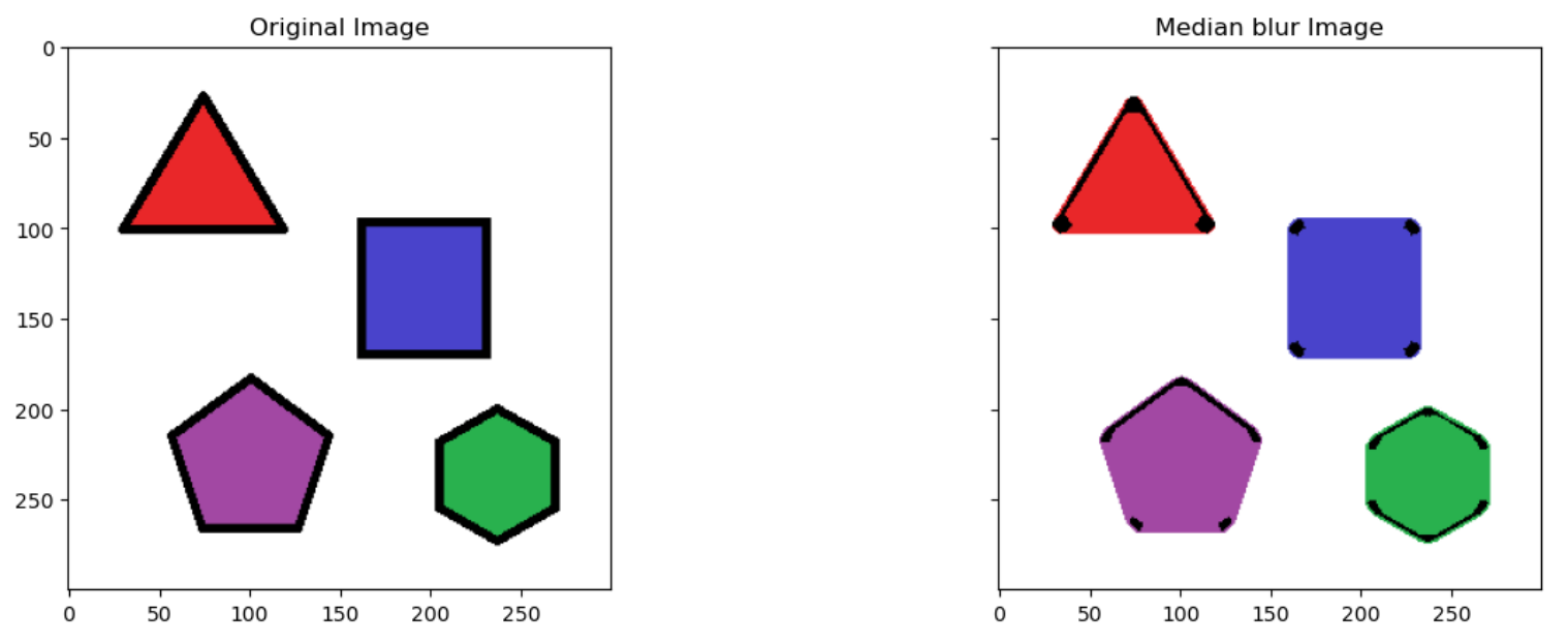
Median Filter: img = cv.imread('../input/images-for-computer-vision/simple_shapes.png') # Median Filter ksize = 11 img_medianblur = cv.medianBlur(img, ksize) myplot([img, img_medianblur], ['Original Image', 'Median blur Image'])
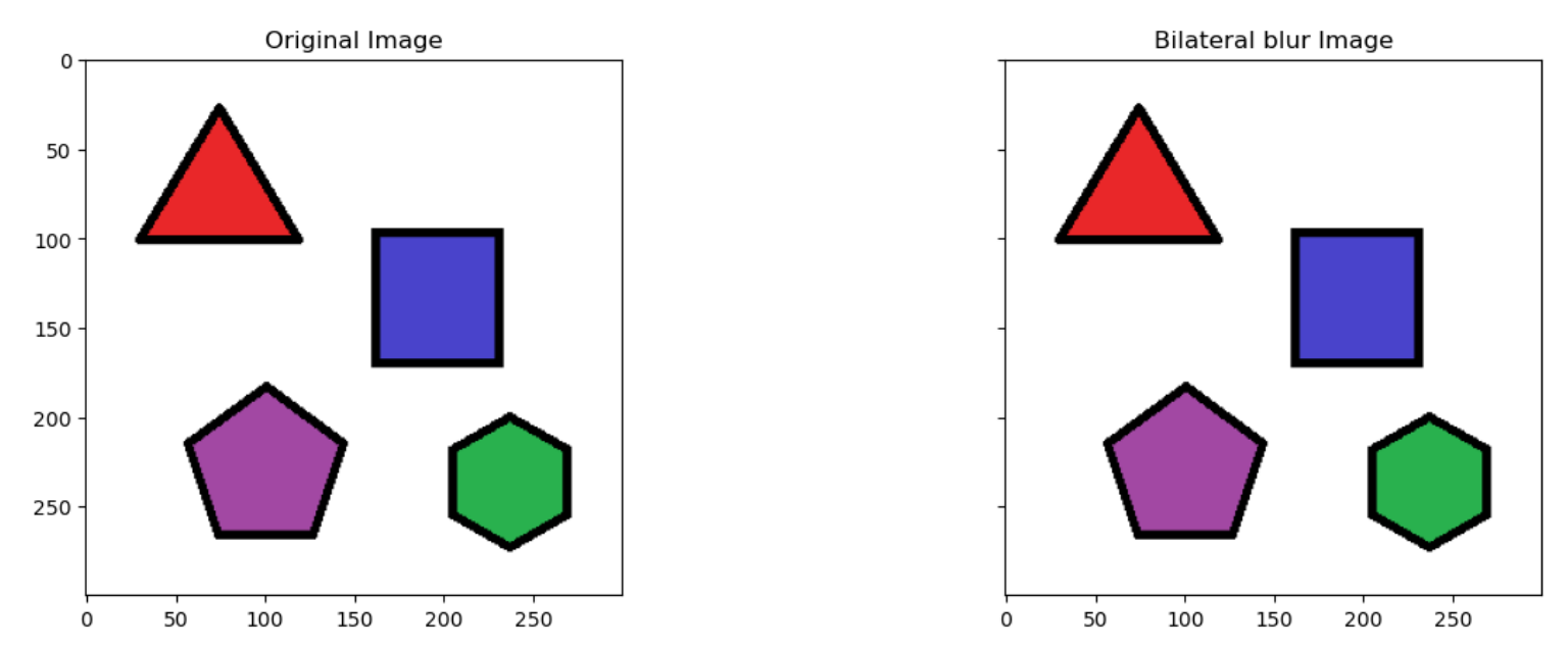
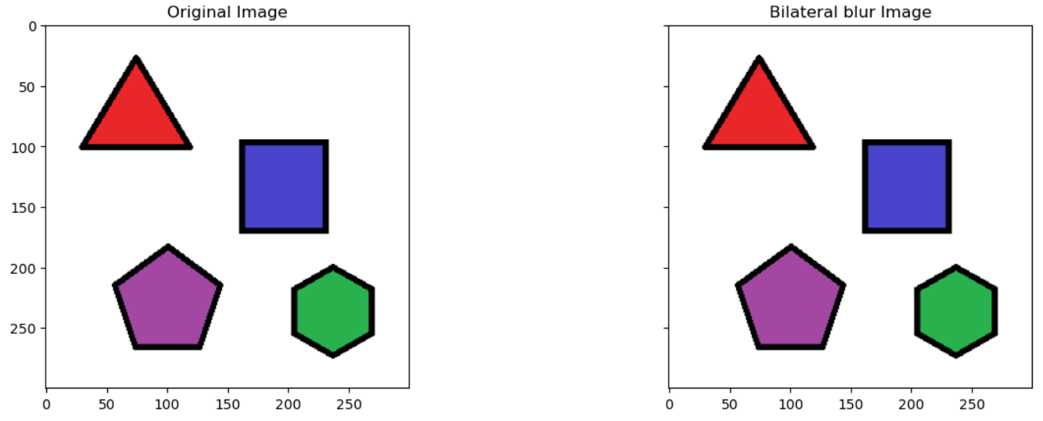
Bilateral Filter: img = cv.imread('../input/images-for-computer-vision/simple_shapes.png') # Bilateral Filter img_bilateralblur = cv.bilateralFilter(img, d = 5, sigmaColor = 50, sigmaSpace = 5) myplot([img, img_bilateralblur],['Original Image', 'Bilateral blur Image'])
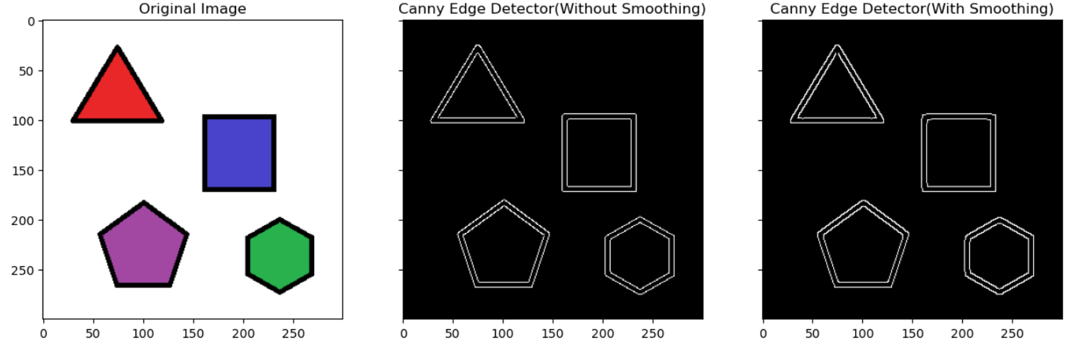
特征检测是计算机视觉领域中的一项重要任务,旨在从图像或图像序列中自动识别和定位具有特定属性或结构的显著特征。这些特征可以是图像中的角点、边缘、纹理、颜色区域等。特征检测的目标是从输入的图像数据中提取出具有独特性、稳定性和可区分性的特征点或特征描述子。 特征检测在许多计算机视觉任务中都起到关键作用,例如目标识别、图像配准、运动跟踪、图像拼接等。它提供了一种有效的方式来描述和表示图像中的关键信息,从而实现对图像内容的理解和分析。 特征检测算法通常包括以下步骤: 尺度空间构建:通过使用尺度空间(例如高斯金字塔)来检测不同尺度下的图像特征,以应对图像中物体的尺度变化。响应计算:使用适当的滤波器或算子在图像上计算特征响应,以找到潜在的特征点位置。特征点筛选:对响应图像进行非极大值抑制或其他筛选方式,以选择最具代表性的特征点。特征描述:对选定的特征点进行描述,生成能够描述其局部外观和结构的特征描述子。常见的特征检测算法包括Harris角点检测、SIFT(尺度不变特征变换)、SURF(加速稳健特征)和ORB(Oriented FAST and Rotated BRIEF)等。这些算法采用不同的方法来寻找、描述和匹配图像中的特征点,根据具体任务和应用场景的需求选择适合的算法。 特征检测的优点在于其对于光照、尺度、旋转和视角的变化具有一定的不变性,能够提供稳健的特征表示,从而在计算机视觉领域中广泛应用。 import numpy as np import pandas as pd import plotly.express as px img = cv.imread('../input/images-for-computer-vision/simple_shapes.png') img_canny1 = cv.Canny(img,50, 200) # Smoothing the img before feeding it to canny filter_img = cv.GaussianBlur(img, (7,7), 0) img_canny2 = cv.Canny(filter_img,50, 200) myplot([img, img_canny1, img_canny2], ['Original Image', 'Canny Edge Detector(Without Smoothing)', 'Canny Edge Detector(With Smoothing)'])
|

 Gaussian Filter:
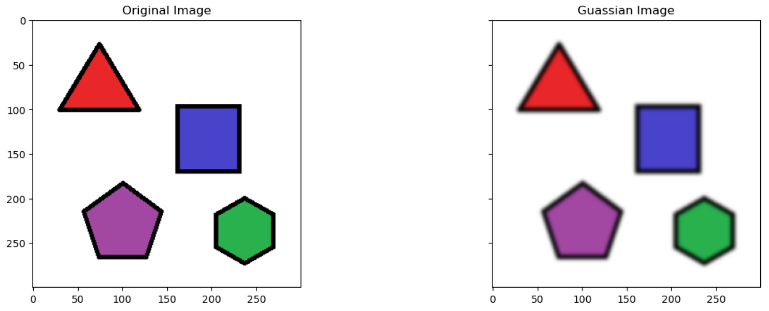
【本文地址】